An autonomous polynomial ODE with six state variables, started once and left to run, has π as its only stable equilibrium.

A postcard from Madras

In 1914, a young clerk in the Madras Port Trust accounts office, with little more than a battered copy of G. S. Carr’s Synopsis of Pure Mathematics, sent a paper to the Quarterly Journal of Mathematics that contained a list of seventeen formulas for $1/\pi$. Each was startling. The simplest of them was

Even the first term already gives $1/\pi$ to eight decimal places, and each additional term adds another eight. Ramanujan did not prove any of the seventeen formulas. It took seven decades and two Borwein brothers to put them on a rigorous footing, by way of modular forms of level four and a K3 family of elliptic surfaces.

This post does something smaller and more concrete. It asks: can the right-hand side of the formula above be computed by an analog machine — more precisely, by a general-purpose analog computer (GPAC) in the sense of Shannon (1941), extended by Bournez, Campagnolo, Graça, and Hainry? The answer is yes, with a six-dimensional polynomial ODE. The rest of this post constructs that ODE, explains where each equation comes from, and watches the machine converge to $\pi$ in a simulation.

The coefficients are holonomic

Write the Ramanujan coefficient as $a_k := (4k)!/(k!)^{4}$. A direct computation on the ratio $a_{k+1}/a_k$ gives

Equation (1) is the defining feature of the Ramanujan series. It says the ratio of consecutive coefficients is a rational function of $k$. Sequences with this property are called P-recursive, or equivalently holonomic: their generating function satisfies a linear ODE with polynomial coefficients.

Introduce the generating function

Using the Euler operator $\theta := z\, d/dz$ (which acts on $z^k$ by multiplication by $k$), the recurrence (1) translates into an ODE essentially by inspection. The cube $(k+1)^{3}$ corresponds to $\theta^{3}$ applied to $\sum a_{k+1} z^{k+1}$; the cubic polynomial $(4k+1)(4k+2)(4k+3)$ equals $64\,(k+\tfrac14)(k+\tfrac12)(k+\tfrac34)$, which corresponds to $64\,(\theta+\tfrac14)(\theta+\tfrac12)(\theta+\tfrac34)$. The extra factor of $4$ and the shift from $z^{k}$ to $z^{k+1}$ combine into $256\, z$. The result is

This is the Clausen hypergeometric equation for ${}_{3}F_{2}(\tfrac14,\tfrac12,\tfrac34;\,1,1;\,256 z)$. It has three singular points: $z=0$, $z=1/256$, and $z=\infty$. At $z=0$ the indicial polynomial is $\rho^{3}$, a triple root at zero — the point of maximum unipotent monodromy (often abbreviated MUM). The analytic solution at this singularity is the $f(z)$ we started with, with $f(0)=1$; the other two solutions involve $\log z$ and $(\log z)^{2}$ and are irrelevant here.

Converting (2) from Euler form to ordinary derivatives and clearing a factor of $z$ gives the form we will actually simulate:

Two coefficients of (3) vanish at $z = 0$, reflecting the MUM; one vanishes at $z = 1/256$, the other regular singular point.

Why Ramanujan’s evaluation point is deep interior

The Ramanujan evaluation lives at $z_{0} := 1/396^{4}$. Two things matter about this number.

First, $z_{0}$ is far inside the convergence disk: $z_{0} \approx 4.1 \times 10^{-11}$, while the disk has radius $1/256 \approx 3.9 \times 10^{-3}$. The ratio $256\, z_{0} = 1/99^{4} \approx 1.04 \times 10^{-8}$ is the per-term geometric decay factor of the series at $z_{0}$.

Second, a short manipulation shows that Ramanujan’s series is precisely the evaluation of a linear combination of $f$ and $z f'$ at $z = z_{0}$:

So once we can evaluate $f(z_0)$ and $f'(z_0)$, formula (4) hands us $1/\pi$ directly.

The GPAC model: why polynomial ODEs

A general-purpose analog computer, in Shannon’s formulation, is a network of adders, multipliers, integrators, and constants. The functions computable by a GPAC are exactly the solutions of polynomial initial value problems (PIVPs):

where each $p_{i}$ is a polynomial. If the PIVP has an exponentially stable equilibrium at a value $x^{\star}$, then starting the machine anywhere in the basin of attraction, one reads off $x^{\star}$ asymptotically. The theorem of Bournez–Campagnolo–Graça–Hainry (2007) says this model is polynomial-time equivalent to Turing machines. The subclass with bounded state spaces corresponds to a complexity class of real numbers — the setting in which a ζ(3)- or π-computing machine can be studied as a concrete, low-dimensional analog circuit.

Our task is to squeeze the Ramanujan route to $\pi$ into this polynomial-RHS straitjacket.

A change of variable to set the stage

The straightforward impulse is to integrate equation (3) from some $z_{1}>0$ to $z_{0}$. That turns out to be numerically awkward because $z_{0}$ is close to the MUM point $z=0$, where the $z^{2}$ factor on the left of (3) makes the ODE degenerate.

A cleaner choice is to rescale: set

Then $g(0) = f(0) = 1$, $g(1) = f(z_{0})$, $g'(1) = z_{0} f'(z_{0})$, and a direct chain-rule calculation converts (3) into an ODE for $g$ on $[0,1]$ with the same structure but rescaled coefficients:

The MUM at $w=0$ is unchanged; the other regular singular point has moved from $z=1/256$ to $w = 1/(256\, z_{0}) = 99^{4} \approx 10^{8}$, far outside our interval $[0,1]$. Formula (4) becomes simply

Building the six-state GPAC

The remaining challenge is that (5) contains the non-polynomial factor $1/[w^{2}(1 - 256\, z_{0}\, w)]$ when solved for $g'''$. Shannon’s GPAC does not permit division, so we must eliminate this denominator.

The standard trick is to add the reciprocal as a new state variable. Let

and treat $Q$ as a degree of freedom on equal footing with $g$. Its derivative with respect to $w$ is, by the quotient rule,

which is polynomial in $(w, Q)$ — denominators gone.

Next, we time-rescale. The simulation needs to steer $w$ from near $0$ to $w=1$. The cleanest GPAC-compatible driver is the linear relaxation

This has $w = 1$ as a globally exponentially stable fixed point with decay rate $1$. Composing with the $w$-ODE (5), every derivative of $g$ gets multiplied by the drift $(1-w)$, which is polynomial.

Finally, a readout channel and a closed-loop inverter. Define

By (6), $I(X(\tau)) \to 1/\pi$ as $\tau \to \infty$. To convert $1/\pi$ to $\pi$ without division, introduce one last state variable $P$ obeying

When $I$ equals a constant $c>0$, equation (8) has the exponentially stable fixed point $P = 1/c$ with linearized rate $c$. Since $I(X(\tau)) \to 1/\pi$, the state $P(\tau)$ converges to $\pi$ exponentially at rate $1/\pi \approx 0.318$. The converter is Newton-free: no square roots, no Taylor expansions, just a single first-order linear ODE.

Collecting everything, the GPAC model is the six-dimensional PIVP with state $X = (w, Q, g, g', g'', P)$ and

Every right-hand side is a polynomial in the six state variables. The coefficients are real constants, as GPAC allows. The readout is $\lim_{\tau \to \infty} P(\tau) = \pi$.

Initial conditions are supplied by a truncated Taylor series for $g$ at some small $w_{1} > 0$ (say $w_{1} = 10^{-3}$): from $g(w) = \sum_{k} a_{k} z_{0}^{k} w^{k}$, the first few derivatives at $w_{1}$ can be computed with a handful of terms because the factor $z_{0}^{k}$ shrinks superexponentially. One then sets $Q(0) = 1/[w_{1}^{2}(1 - 256 z_{0} w_{1})]$ and picks any positive $P(0)$ in the basin of the $P$-inverter (for example $P(0) = 3$).

What the simulation sees

Integrating (9) numerically with a standard adaptive Runge–Kutta solver (DOP853, relative tolerance $10^{-12}$) from $\tau = 0$ to $\tau = 60$ produces three clean exponentials (Figure 1, right panel).

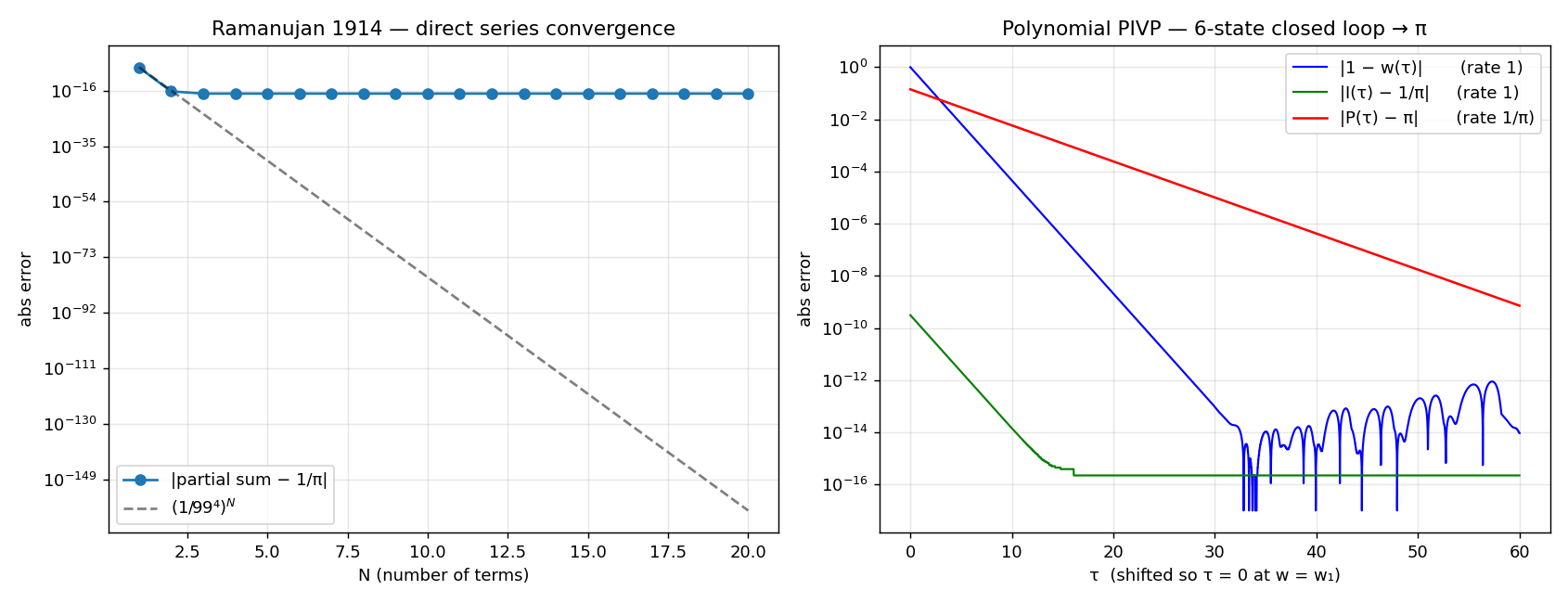
The $w$-trajectory approaches $1$ at rate $1$. The readout $I(\tau)$ approaches $1/\pi$ at the same rate, hitting machine precision around $\tau \approx 30$. The converter $P(\tau)$ approaches $\pi$ at rate $1/\pi \approx 0.318$, the shallower slope in the plot — slower only because the linearization of (8) is limited by the magnitude of $I$ itself. At $\tau = 60$ one has $|P(\tau) - \pi| \approx 7 \times 10^{-10}$; the remaining gap is bounded only by the rate-$1/\pi$ geometry of (8), not by Ramanujan’s series.

The left panel shows, for contrast, the discrete partial sums of Ramanujan’s original series. Two terms already give sixteen correct decimals; three terms saturate double-precision. The geometric dashed line $(1/99^{4})^{N}$ traces the theoretical per-term envelope. The series itself is not what our GPAC runs — the GPAC runs the continuous flow — but the discrete plot is useful as a sanity check and as a reminder of how far into the convergence disk the Ramanujan point sits.

Fitted slopes from the simulation match the theory to three or four decimals: rate $\alpha \approx 0.99$ for $w$ and $I$ (theory: $1$), and $\alpha \approx 0.318$ for $P$ (theory: $1/\pi = 0.3183$).

The shape of the construction

Three mechanisms do the work.

A holonomic substrate. The coefficients $a_{k} = (4k)!/(k!)^{4}$ are holonomic because their ratio is rational in $k$. This is not special to Ramanujan — it is true of every hypergeometric series, and more generally every sequence governed by a P-recurrence. The Picard–Fuchs ODE (3) is the algebraic shadow of that property, and the only reason the analog machine can exist at all.

A domain rescaling. The Ramanujan evaluation point $z_{0}$ sits awkwardly close to the MUM singularity at zero. Pulling it out to $w = 1$ moves the action away from the numerically bad part of the complex plane, at the cost of nothing structural — the ODE’s shape is preserved.

Polynomialisation. Two tricks convert the resulting linear ODE into a polynomial PIVP: carrying $1/[w^{2}(1 - 256 z_{0} w)]$ as an extra state, and using $dw/d\tau = 1 - w$ to absorb the division by that factor. These two moves are generic — they work for any linear ODE with polynomial coefficients — and so the whole construction carries over to every hypergeometric series with a rational evaluation point inside its convergence disk.

A closed-loop converter. The linear inverter $\dot P = 1 - I P$ is cheaper than one might expect. It uses no Newton iteration, no explicit division; its only ingredients are a multiplication and a subtraction. The price is a convergence rate equal to the target value (here, $1/\pi$), which is not usually a problem for hypergeometric targets.

Why this is interesting

The Ramanujan series is sometimes told as a story about modular forms, and sometimes as a story about super-fast π computation. It is worth telling once as a story about analog computation. The formula is old; the analog interpretation is not. What the six-state PIVP (9) makes precise is the following claim:

there exists a smooth, autonomous, bounded, six-dimensional polynomial vector field on $\mathbb{R}^{6}$ whose unique attractor is a point whose last coordinate is $\pi$.

The geometry of the construction mirrors the mathematical content. The MUM at $z = 0$ is why a variable change is needed; the holonomic ratio is why the ODE exists; the polynomial-PIVP straitjacket is why the reciprocal-state and time-rescaling tricks appear. The 1103 and 26390 that made Ramanujan’s formula look like numerology are, in this picture, simply the coefficients of a one-parameter family of linear combinations of $g$ and $g'$ that happen to land on $1/\pi$.

A reader with a fondness for physical metaphors may read the last state $P$ as the output pin of the circuit. Everything upstream is a hypergeometric generator; $P$ is the meter. And the meter is settling.

All code and plots are in projects/Ripple/experiments/ramanujan1914_pivp.py. The Lean 4 scaffolding that verifies the recurrence (1) and the coefficient form of the ODE (2) is in projects/Ripple/Ripple/Number/Ramanujan1914.lean; Ramanujan’s identity (6) itself remains open there, as it rightly should — the serious Borwein-style proof via modular forms is a separate undertaking.

大衍之数五十，其用四十有九。—《易·系辞》

Of the fifty stalks of the great divination, forty-nine come into use.