Tunable-Rate Inverters for Analog Reciprocal Computation
2026-04-24
A continuation of the previous two posts on the Ramanujan circuit. The linear inverter $\dot P = 1 - I\,P$ — the standard polynomial trick for turning an analog estimate of $1/\pi$ into one of $\pi$ — relaxes at rate $I_\infty = 1/\pi \approx 0.318$, slower than every other module upstream. It need not. Replacing it with a one-line variant $\dot P = P\bigl(1 - (I\,P)^k\bigr)$ raises the asymptotic rate to any positive integer $k$, with no extra state and no extra constants. The upstream chain stays the bottleneck again, where it ought to be.
What the previous posts left on the table
The previous post ended with a $\sim 10^{-12}$ readout for $\pi$ at $\tau = 60$, two orders of magnitude better than the original construction. The improvement came from rerouting the circuit so that the inverter sees the large quantity $T_\infty := 1103\,g_\infty + 26390\,g'_\infty \approx 1103$ rather than its small reciprocal $1/\pi$. An inverter $\dot L = 1 - T\,L$ relaxes at rate $T_\infty$; relax fast, multiply by the rational and irrational scalars at the end, and the slow $1/\pi$ rate drops out.
That is one structural fix. There is another, which deserves to be said cleanly on its own. The linear inverter has a fixed asymptotic rate equal to the value of its coefficient. If the natural quantity the circuit hands you to invert really is small — really is on the order of $1/\pi$ — there is nothing to reroute, and the linear inverter’s rate is what you get. So: is there a different polynomial inverter, with the same asymptotic value, but a faster relaxation rate?
There is. The construction below is one line of state per inverter. It introduces no new constants, no new variables, and stays inside the class of polynomial ODEs with rational coefficients. The asymptotic rate becomes a free parameter $k \in \mathbb{Z}_{\ge 1}$, recovering the standard linear inverter at $k = 1$ and continuous Newton flow at $k = 1$ as well (they are the same thing under a translation).
A caveat first, since the previous post raised the question explicitly: this trick still computes $\pi$ by inverting an analog estimate of $1/\pi$. It speeds up the inverter, but it does not bypass inversion. The genuinely interesting open question — can $\pi$ be extracted directly from the holonomic series for $1/\pi$ without passing through $1/\pi$ as an intermediate variable? — is the subject of a future post.
The standard inverter and what limits it
Given an upstream signal $I(\tau) \to I_\infty$, the linear inverter is
This is the simplest polynomial PIVP module that solves the algebraic equation $I \cdot P = 1$. Asymptotically, with $I(\tau) \approx I_\infty$, the deviation $\delta P := P - P_\infty$ satisfies
so $\delta P$ decays at rate exactly $I_\infty$. There is no choice of initial condition or transient that can do better; the rate is set by the linearisation, not by the initial slope. In the Ramanujan circuit this rate is $I_\infty = 1/\pi$, and it is the slowest module in the chain.
Reframing: Newton flow
Write $\dot P = 1 - I\,P = -I(P - 1/I)$ and rescale time by $1/I$. The flow becomes the Newton flow for $f(P) = I\,P - 1$:
The same fixed point, the same exponential rate of $1$ in the rescaled time $s$. The standard linear inverter is exactly Newton flow on the linear equation $I\,P = 1$, with the time-rescaling absorbed into the coefficient. The rate $I_\infty$ is the cost of not rescaling.
Now consider the equivalent formulation that does not rely on the multiplier in front:
Here the right-hand side is still polynomial in $(I, P)$, with no explicit dependence on $1/I$. Two fixed points: $P = 0$ and $P = 1/I$. Linearising at $P_\infty = 1/I$ gives
so the asymptotic rate is now $1$, independent of the value of $I$. That is the first improvement: trading $\dot P = 1 - I\,P$ for $\dot P = P\,(1 - I\,P)$ changes the rate from $I_\infty$ to $1$. In the Ramanujan circuit, that is a factor-$\pi$ speedup at no extra cost.
Tuning the rate: logistic-$k$ flow
The next observation is that nothing in the linearisation argument prevents us from raising the nonlinearity. Consider
Still polynomial in $(I, P)$, still degree only $k+1$ — and crucially, still with no extra state and no irrational constants beyond whatever $I$ already contains. Substitute $x := I\,P$ (assuming $I$ is asymptotically constant, which it is); then
a logistic-$k$ ODE with stable fixed point $x = 1$. Linearising $h(x) := x(1 - x^k)$ at $x = 1$:
The asymptotic rate of $\delta x$, and hence of $\delta P = \delta x / I$, is exactly $k$. So the inverter rate becomes a tunable parameter: take $k = 1$ for Newton flow, $k = 2$ for cubic flow, $k = 3$ for quartic, and so on. The asymptotic value of $P$ is $1/I_\infty$ for every $k$ — only the speed of approach changes.
What this is not: not Householder’s method
The previous version of this post called the rate-$k$ flow a continuous analogue of Householder’s method, and that was wrong. The correction is worth stating carefully because the two ideas are easy to confuse and they live in different complexity worlds.
Householder’s method for solving $f(P) = 0$ is a discrete iterative scheme
whose hallmark is order of convergence: the per-step error obeys $|P_{n+1} - P_*| = O\bigl(|P_n - P_*|^{d+1}\bigr)$, which is quadratic for $d = 1$ (the classical Newton iteration), cubic for $d = 2$, and so on. The order $d + 1$ is what people quote when they sell Householder.
Now take any of these schemes to a continuous flow by $P_{n+1} - P_n \approx \Delta\tau\,F_d(P_n)$. The vector field $F_d$ is, for every $d$, of the form
so its linearisation at $P_*$ — where $f(P_*) = 0$ — is just $-(P - P_*)$. Every continuous Householder flow linearises at the same rate, namely $1$. The high-order convergence of the discrete scheme is a property of finite step size; in the continuous limit it washes out. There is no “rate $d+1$” continuous Householder flow.
That is why the speedup of the rate-$k$ inverter cannot be Householder in disguise. The rate-$k$ flow is not a Newton-type flow at all in the sense of “find the zero of $f$ by following $-f/f'$.” It is a deformation of the right-hand side itself, raising the nonlinearity from $1 - I\,P$ to $1 - (I\,P)^{k}$. The change of variable to $x = I\,P$ exposes it as a logistic-$k$ ODE — a one-line fact about super-attracting fixed points of polynomial flows on the line, with no nonlinear-rootfinding heritage.
A useful test: the standard discrete Newton iteration $P_{n+1} = P_n + (1 - I\,P_n)/I$, run with step $\Delta\tau \to 0$, gives the linear inverter $\dot P = 1 - I\,P$ — rate $I$. The discrete Newton iteration $P_{n+1} = P_n + P_n(1 - I\,P_n)$ (a different algebraic manipulation of the same root condition) gives, in the same limit, $\dot P = P(1 - I\,P)$ — rate $1$. Both are continuous Newton flows in the sense of $f' \neq 0$, and the rate difference comes from the algebraic form of the discrete scheme, not from any higher-order derivative information. Householder simply doesn’t enter.
Numerical check on the Ramanujan circuit
The plot below plugs the rate-$k$ inverter into the same six-state Ramanujan circuit from two posts ago, swapping only the inverter ODE.
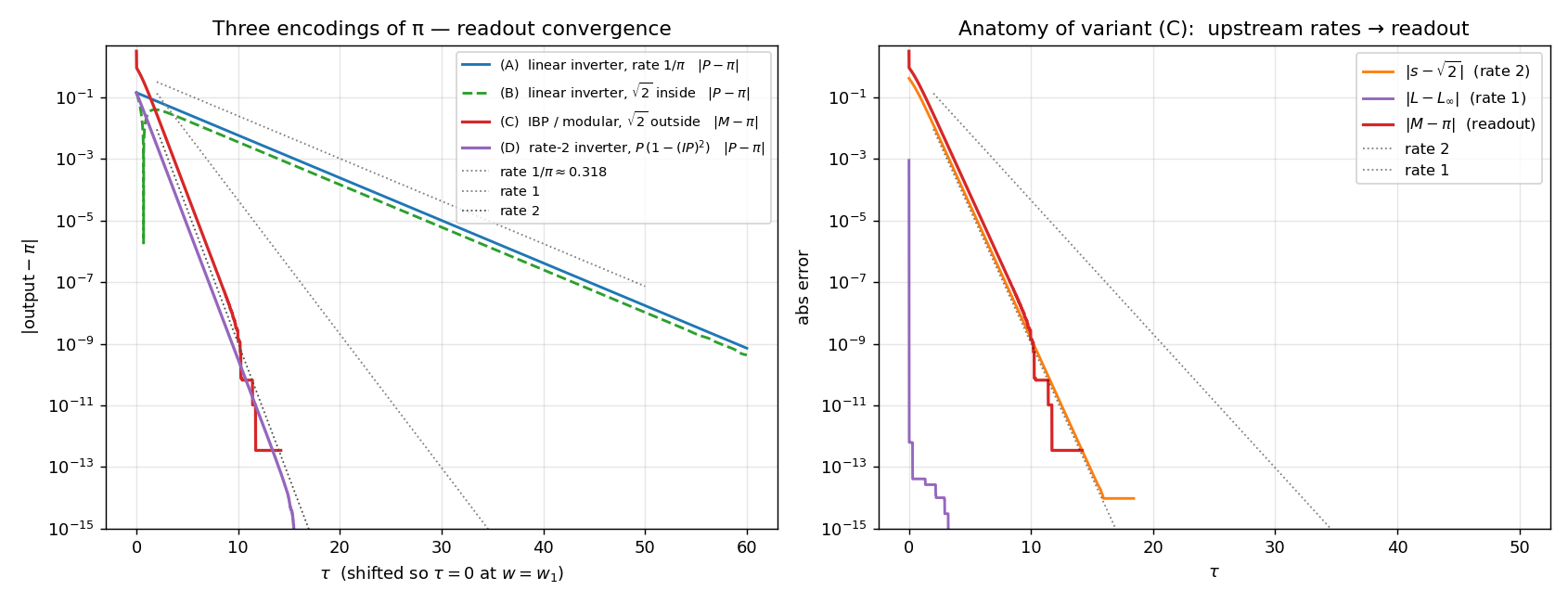
Numerical fits of the asymptotic rate $\alpha$ from $|P(\tau) - \pi| \sim e^{-\alpha\tau}$ on the pre-saturation window:
| $k$ | $\lvert P - \pi\rvert$ at $\tau = 60$ | fitted rate $\alpha$ | expected | window |
|---|---|---|---|---|
| linear inverter | $7.2 \times 10^{-10}$ | $0.318$ | $1/\pi$ | $\tau \in [8, 55]$ |
| 1 (Newton flow) | $6.5 \times 10^{-14}$ | floor reached | $1$ | saturates by $\tau \approx 30$ |
| 2 (cubic flow) | $4.0 \times 10^{-15}$ | $\boxed{2.0005}$ | $2$ | $\tau \in [4, 12]$ |
| 3 (quartic flow) | $2.5 \times 10^{-13}$ | floor reached | $3$ | saturates by $\tau \approx 3$ |
| 4 (quintic flow) | $1.8 \times 10^{-15}$ | floor reached | $4$ | saturates by $\tau \approx 3$ |
The $k = 2$ case has a genuine measurable rate window before saturation, and the fitted slope is within $0.025\%$ of the predicted $2$. For $k = 3$ and $k = 4$ the readout reaches the double-precision floor in just a few units of $\tau$ — the rate is high enough that there is no measurable exponential window left in finite-precision arithmetic. The fitted slopes for those rows are noise. The point of including them in the table is precisely to illustrate the saturation: by the time you can observe the trajectory, the answer is already as accurate as the arithmetic allows.
The $k = 1$ row is qualitatively different from the linear inverter row even though both have asymptotic rate $1$ in the relevant variable. Why? Because for the linear inverter, $\dot P = 1 - I\,P$, the rate in $P$ itself is $I_\infty = 1/\pi$, not $1$. The $k = 1$ flow, $\dot P = P(1 - I\,P)$, has rate $1$ in $P$. They differ by exactly the factor $1/\pi$ in their linearisation, and that factor is what the plot is showing.
What this buys, and what it doesn’t
What it buys:
- A single-line fix. The change is one polynomial right-hand side of degree $k+1$; no new state, no new constant, no irrational coefficient introduced.
- A free choice of rate. The asymptotic rate of any inverter in the polynomial-PIVP world is now whatever positive integer one wants. In the Ramanujan circuit this turns the inverter from the slowest module into one of the fastest.
- The bottleneck moves back upstream where it should be. With a rate-$2$ or higher inverter, the limiting rate of the readout is set by the upstream holonomic dynamics — by the convergence of the Picard–Fuchs ODE — not by an artefact of the polynomial-PIVP machinery used to invert.
What it does not buy:
- It does not bypass inversion. The circuit still computes $1/\pi$ first and then inverts. The truly direct route — extract $\pi$ from the holonomic series for $1/\pi$ without passing through $1/\pi$ as an intermediate variable — remains open.
- It does not surpass arithmetic precision. The $k = 3$ and $k = 4$ variants saturate at the double-precision floor too quickly to display their advertised rates. In any setting with finite precision, there is a $k$ above which extra rate is wasted.
- It does not change asymptotic complexity. Polynomial-PIVP complexity classes are typically defined up to multiplicative factors in the rate; raising the rate by an integer $k$ keeps the construction in the same class. The improvement is constant-factor from a complexity-class standpoint, but it is the difference between a usable and an unusable circuit in any given precision.
The third point in particular is worth dwelling on. The inverter is not a bottleneck because it has a slow rate in principle; it is a bottleneck because the natural value of its coefficient happens to be $1/\pi$, which is a small number. The rate-$k$ trick makes the inverter rate independent of that coefficient, restoring the expected hierarchy: holonomic dynamics set the pace, the rest of the circuit follows. The complexity class doesn’t change, but the shape of the convergence does — and shape is what determines whether a polynomial-PIVP circuit produces useful digits in a given run.
Where this fits in the Ramanujan trilogy
Three posts, three structural choices. The first introduced the six-state circuit and observed that the linear inverter dominates the relaxation rate. The second pulled $\sqrt{2}$ outside the inverter, so that the inverter sees a large quantity instead of $1/\pi$, and made the integration-by-parts modular composition explicit. This post closes the loop on the inverter itself: even when the natural quantity is small, a one-line modification of the inverter ODE removes that quantity from the asymptotic rate.
Together these are three independent levers — circuit topology (routing $\sqrt{2}$), module choice (which inverter ODE), and time parametrisation. A clean polynomial-PIVP construction tends to need all three. The fourth lever, which removes inversion altogether by returning to the holonomic series in a form that yields $\pi$ directly, is the next post.
穷则变,变则通,通则久。 — 《周易·系辞下》
“When something reaches its limit it must change; once changed, it flows; and once it flows, it endures.” — Book of Changes, Great Treatise II.