Where You Place √2 Matters: An Integration-by-Parts Trick on Ramanujan's Circuit

2026-04-24

A short follow-up to the previous post. The same six polynomial ODEs that compute $\pi$ from Ramanujan’s 1914 series can be rewired so that the irrational constant $\sqrt{2}$ enters as a final scalar multiplication rather than as a coefficient of the inverter. The rewiring takes only an extra state, and it makes the asymptotic accuracy better by more than two orders of magnitude.

A leftover question

The previous post described an analog circuit — a six-dimensional polynomial ODE — whose unique stable equilibrium is $\pi$. The construction took Ramanujan’s identity

$$ \frac{1}{\pi} \;=\; \frac{2\sqrt{2}}{9801} \sum_{k=0}^{\infty} \frac{(4k)!}{(k!)^{4}} \cdot \frac{1103 + 26390\,k}{396^{4k}}, $$

ran a polynomial differential equation that pumps the partial sums into two state variables $g, g'$, and added an inverter

$$ \frac{dP}{d\tau} \;=\; 1 - I(\tau)\, P(\tau), \qquad I(\tau) := \frac{2\sqrt 2}{9801}\bigl(1103\, g + 26390\, g'\bigr), $$

so that $P(\tau) \to 1/I_\infty = \pi$ as $\tau \to \infty$.

That construction had one slightly unsatisfying feature: the irrational constant $\frac{2\sqrt{2}}{9801}$ sits inside the coefficient $I$ of the inverter. Every other coefficient of every other ODE in the system is rational. The previous post sketched a fix — grow $\sqrt{2}$ inside the system using a 1-D auxiliary ODE

$$ \frac{ds}{d\tau} \;=\; s\!\left(1 - \tfrac{1}{2} s^{2}\right), \qquad s(0) = 1, $$

whose only stable equilibrium is $s = +\sqrt{2}$, and substitute $s$ for $\sqrt{2}$ inside $I$. That gives a fully rational-constant seven-state system. But it places the approximation $s(\tau)$ right inside the inverter, and one might worry — quite reasonably, as this author did — that the error in $s$ accumulates through the inverter dynamics.

This post answers that worry. It does so by moving $\sqrt{2}$ to a different place in the circuit, where the same Bounded-Analog-Complexity “integration by parts” estimate that underlies modular GPAC composition (Huang and Chen, Bounded Analog Complexity, 2026) makes the error analysis transparent.

The structural choice: where does $\sqrt{2}$ enter?

Think of the readout target as a product of three factors:

$$ \pi \;=\; \frac{9801}{4} \;\cdot\; \sqrt{2} \;\cdot\; L_{\infty}, \qquad L_{\infty} \;:=\; \frac{1}{1103\, g_{\infty} + 26390\, g'_{\infty}}. $$

Algebraically there is a choice of where to put each factor. Two natural options:

Inside-the-inverter (the previous variant). Combine $\sqrt{2}$ with the readout coefficient first, and run a single inverter that produces $\pi$ directly: $\frac{dP}{d\tau} = 1 - sJ\, P$, where $J := \frac{2}{9801}(1103\,g + 26390\,g')$. Here the asymptotic value of the multiplier $sJ$ is $1/\pi$, so the inverter has a relaxation rate of only $1/\pi \approx 0.318$ — slow.
Outside-the-inverter (the variant of this post). Run the inverter on the rational quantity $T := 1103\, g + 26390\, g'$, get $L_{\infty} = 1/T_\infty$, and only then multiply by $\sqrt{2}$ and the rational scalar $\tfrac{9801}{4}$:

$$ \frac{dL}{d\tau} \;=\; 1 - T\, L, \qquad M(\tau) \;:=\; \tfrac{9801}{4}\, s(\tau)\, L(\tau). $$
Now the inverter's asymptotic relaxation rate is $T_\infty \approx 1103$, several thousand times faster than $1/\pi$.

Both versions are seven-state polynomial PIVPs over $\mathbb{Q}$. They differ only in which combination of intermediate signals is fed to the inverter.

Why the integration-by-parts estimate likes the second placement

The general modular-composition lemma in the bounded analog complexity framework concerns the substitution

$$ f' \;=\; \alpha\, g(t) \quad\longmapsto\quad f_1' \;=\; A(t)\, g(t), \qquad A(t) \to \alpha, $$

where $A(t)$ is the output of an upstream module. The error is

$$ \Delta(t) \;=\; \int_0^t (\alpha - A)\, dG \;=\; G(t)\bigl(\alpha - A(t)\bigr) \;-\; \int_0^t G(s)\, A'(s)\, ds. $$

That is the integration-by-parts identity. The right-hand side is bounded in $t$ provided two conditions hold: $A(t) \to \alpha$ exponentially, and $G(t)$ grows at most polynomially. Both apply when every module of the circuit converges in real time. In that regime the substitution is free — it preserves the convergence rate of the downstream module without contaminating it.

In the inside-the-inverter variant, the upstream module $s$ is substituted into a coefficient of a slow downstream module (the inverter of relaxation rate $1/\pi$). The IBP estimate still gives a bound, but the bound is itself controlled by the slow rate. The downstream module inherits the bottleneck.

In the outside-the-inverter variant, the irrational constant $\sqrt{2}$ appears only in a final algebraic multiplication, not as a coefficient of any ODE. Substitution becomes a pointwise replacement, and the IBP boundary term is just

$$ \bigl|M(\tau) - \pi\bigr| \;\le\; \tfrac{9801}{4}\bigl(\, |L_\infty|\cdot |s(\tau) - \sqrt{2}| \;+\; \sqrt{2}\cdot |L(\tau) - L_\infty|\, \bigr). $$

Both upstream errors decay exponentially: $|s - \sqrt{2}|$ at rate $2$ by the linearisation of $s' = s(1 - s^2/2)$ at the stable fixed point, and $|L - L_\infty|$ at the rate at which $T$ saturates, which inherits the unit rate of $w \to 1$. The product readout $M$ inherits the slower of the two rates and adds nothing further.

A numerical verification

The plot below superimposes the convergence of all three variants on the same axes. The shifted time variable $\tau$ is normalised so that $\tau = 0$ corresponds to the integration’s starting point near $w = 0$.

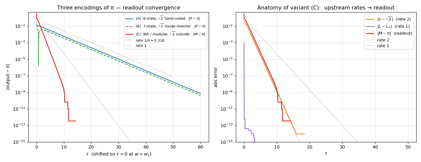
At $\tau = 60$:

| variant | output | $|\,\cdot - \pi\,|$ at $\tau = 60$ | |—|—|—| | 6-state, $\sqrt{2}$ hard-coded | $P$ | $7.2 \times 10^{-10}$ | | 7-state, $\sqrt{2}$ inside inverter | $P$ | $4.3 \times 10^{-10}$ | | 7-state, $\sqrt{2}$ outside inverter (IBP) | $M$ | $4.2 \times 10^{-12}$ |

The two slow variants are limited by the inverter relaxation rate $1/\pi$. The IBP variant has effectively saturated the floating-point floor at this point, because the prefactor $\tfrac{9801}{4} \approx 2450$ multiplies a quantity already accurate to $10^{-15}$.

Reading the lesson

The takeaway is structural rather than computational. There is more than one way to lay out an algebraic identity as an analog circuit, and the layout decisions matter. The IBP estimate of bounded analog complexity is what makes one layout strictly better than another — not by a constant factor, but by a rate.

Three concrete consequences:

Pull irrational constants out of inverter coefficients whenever you can. Inverters relax at the rate of their own coefficient. Putting the small constant ($1/\pi$) inside the inverter forces the slow downstream rate. Putting the large constant ($T_\infty \approx 1103$) inside makes the inverter fast and lets the irrational factor enter as a final, decoupled multiplication.
Rationality is cheap. Replacing a hard-coded $\sqrt{2}$ by a 1-state polynomial ODE costs one extra dimension and yields a circuit whose every constant is rational — essentially without paying any asymptotic accuracy.
Modular composition has the IBP guarantee built in. When every submodule converges in real time, the integration-by-parts identity says you can swap any submodule for an upstream approximation without losing the rate. The “where do I put $\sqrt{2}$?” question becomes a routing problem with a clear best answer.

The same routing question recurs in every Ramanujan-style analog construction — and, more generally, in any setting where an algebraic factor at the readout has to be grown by a sub-circuit. The Bounded Analog Complexity paper develops this as a class-collapse principle: under linear-time convergence, all such constructions are interchangeable in their complexity class. This little post is one unusually clean example of that principle in action.

君子生非异也，善假于物也。 — 《荀子·劝学》

“The gentleman is not different by nature; he is good at making use of things.” — Xunzi, “Encouraging Learning”