Computing Apéry's Constant with Chemistry (Well, Almost)
2026-03-26
How do you compute $\zeta(3) = 1.202056903\ldots$ using only polynomial differential equations? Here’s a construction that does it — and why it matters for chemical computing.
What Is Apéry’s Constant?
Apéry’s constant is the value of the Riemann zeta function at 3:
$$\zeta(3) = \sum_{k=1}^{\infty} \frac{1}{k^3} = 1 + \frac{1}{8} + \frac{1}{27} + \frac{1}{64} + \cdots = 1.2020569031595942\ldots$$Roger Apéry proved in 1978 that this number is irrational — a result so surprising that the mathematical community initially didn’t believe him. The proof was eventually verified and is now considered a landmark of 20th-century number theory.
But we’re not here to prove irrationality. We’re here to compute $\zeta(3)$ — using a system of polynomial ODEs.
Why Polynomial ODEs?
A polynomial initial value problem (PIVP) is a system of ODEs where the right-hand side of each equation is a polynomial in the state variables:
$$\frac{dy_i}{dt} = p_i(y_1, \ldots, y_n), \quad y_i(0) = c_i.$$Why care? Because polynomial ODEs are exactly what chemical reaction networks (CRNs) produce under mass-action kinetics. A reaction $A + B \to C + D$ at rate $k$ contributes $k[A][B]$ to the derivative — a polynomial term. So if you can express a computation as a PIVP, you can (in principle) implement it with chemistry.
Shannon proved in 1941 that polynomial ODEs are the language of analog computation: his General Purpose Analog Computer (GPAC) computes exactly the functions satisfying polynomial ODEs. So a PIVP for $\zeta(3)$ is simultaneously:
- A program for an analog computer,
- A blueprint for a chemical reaction network,
- And a proof that $\zeta(3)$ is “chemically computable.”
The Construction: From Triple Integral to ODE
The starting point is a classical identity:
$$\zeta(3) = \int_0^1 \int_0^1 \int_0^1 \frac{1}{1 - xyz} \, dx \, dy \, dz.$$This follows by expanding $\frac{1}{1-xyz} = \sum_{n=0}^{\infty}(xyz)^n$ and integrating term by term. Beautiful, but a triple integral isn’t an ODE.
Step 1: Reduce to a single integral
Using the Gamma function identity $\frac{1}{k^3} = \frac{1}{2}\int_0^{\infty} t^2 e^{-kt} \, dt$, we can write:
$$2\zeta(3) = \int_0^{\infty} \frac{t^2}{e^t - 1} \, dt.$$This is the standard integral representation, but it has a singularity at $t = 0$ (the integrand blows up). We can’t start an ODE at a singularity.
Step 2: Split and regularize
Split the integral at $t = 1$:
$$2\zeta(3) = \underbrace{\int_0^1 \frac{t^2}{e^t - 1} \, dt}\_{I\_1} + \underbrace{\int_1^{\infty} \frac{t^2}{e^t - 1} \, dt}\_{I\_2}.$$Each piece gets its own change of variables to move the singularity away from the starting point:
For $I_1$: Flip ($t = 1 - s$) then stretch ($s = 1 - e^{-r}$) to get:
$$I_1 = \int_0^{\infty} \frac{e^{-3r}}{e^{e^{-r}} - 1} \, dr.$$The integrand is finite at $r = 0$ (it equals $\frac{1}{e-1}$).
For $I_2$: Just shift ($u = t - 1$):
$$I_2 = \int_0^{\infty} \frac{(u+1)^2}{e^{u+1} - 1} \, du.$$Also finite at the origin.
Step 3: Convert integrands to ODEs
Now the key step. Each integrand can be written as the solution of a polynomial ODE system. The state variables track the components of the integrand, and the integral accumulates in a target variable $s_3$.
System for $I_1$ (4 variables):
where $v(t) = e^{e^{-t}}$ and $u_n(t) = \frac{e^{-nt}}{v(t) - 1}$.
System for $I_2$ (3 variables):
where $r(t) = \frac{1}{1 - e^{-(t+1)}}$ and $w_n(t) = \frac{(t+1)^n}{e^{t+1} - 1}$.
Step 4: The complete system
Combine everything and add the accumulator:
Result: $\displaystyle\lim_{t \to \infty} s_3(t) = \zeta(3)$.
Eight variables. Eight polynomial ODEs. That’s all it takes.
Does It Work?
Yes. Here’s a numerical simulation using 4th-order Runge-Kutta:
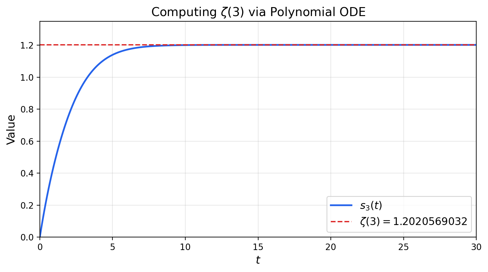
The blue curve is $s_3(t)$, the dashed red line is $\zeta(3) = 1.2020569031\ldots$. By $t = 30$, the error is about $2.4 \times 10^{-11}$.
Here’s what all the species look like over time:
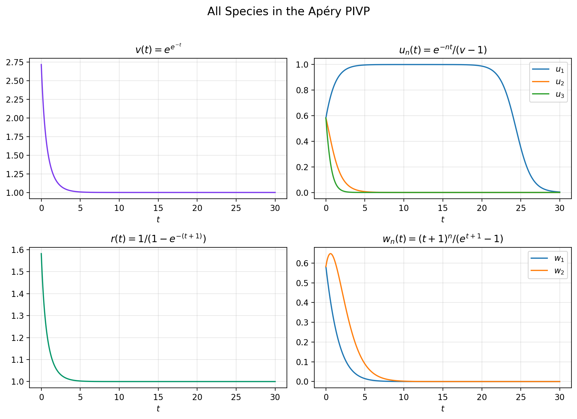
The $u_n$ variables decay exponentially (they’re tracking $e^{-nt}/(v-1)$), while $r$ converges to 1 and $w_n$ converges to 0. The integrand contributions die out, and $s_3$ stabilizes at the answer.
And the error on a log scale:
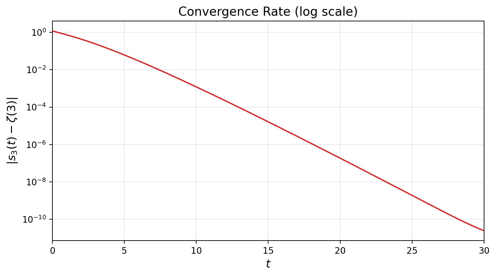
Exponential convergence — roughly one digit of accuracy every 3 units of time.
The Catch: Initial Values
You might have noticed that the initial values involve $e$ and $\frac{1}{e-1}$. These are transcendental numbers — you can’t just “set” a chemical concentration to exactly $e$.
This matters more than it might seem. Think of Turing’s definition of computable numbers: a Turing machine starts with an empty tape. The computation begins from nothing — you don’t get to pre-load the tape with useful information. Similarly, if we want to say a number is “CRN-computable,” we should start from simple initial conditions (say, all zeros or small integers), not from transcendental constants that themselves require computation.
Can we zerolize?
The idea is natural: build an auxiliary ODE system that computes the needed constants dynamically:
This E-block converges beautifully:
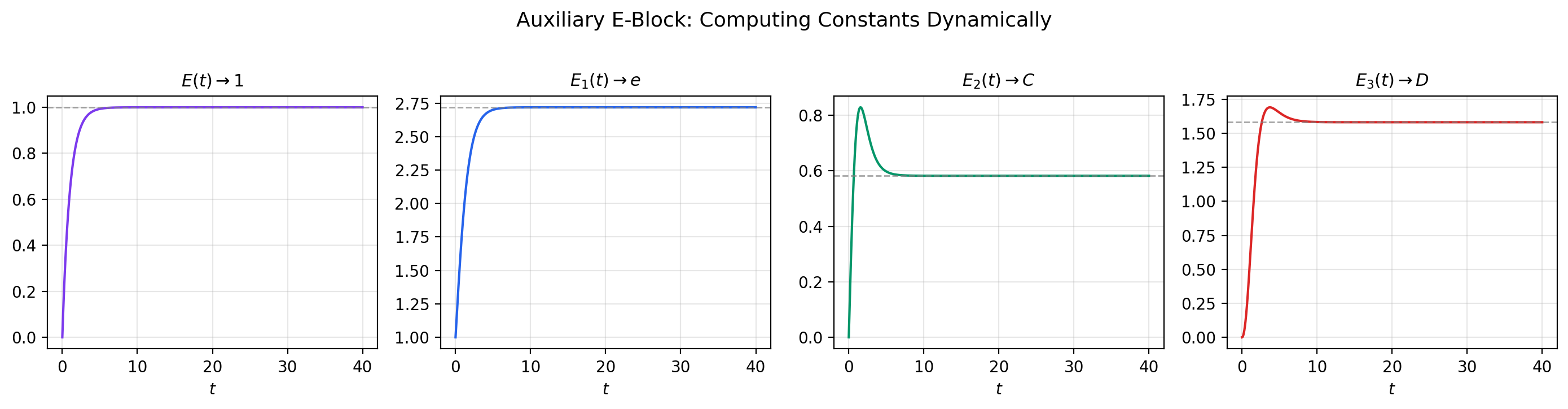
Then plug these dynamical estimates into the main system in place of the true constants $e$, $C = \frac{1}{e-1}$, $D = \frac{e}{e-1}$.
It doesn’t work.
Here’s the plot. The blue curve is the original system (with true initial values). The red curve is the fully zerolized system (E-block replaces all constants):
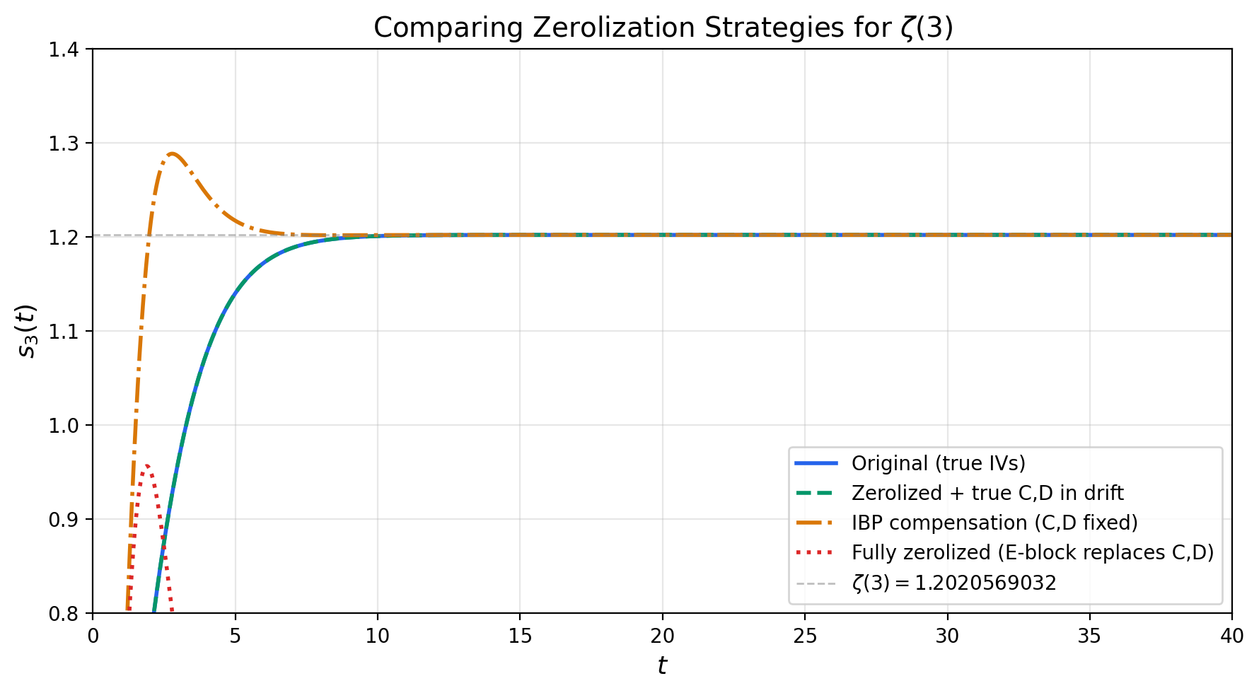
The original converges to $\zeta(3) = 1.2020569\ldots$ The fully zerolized system converges to approximately $0.426$ — completely wrong.
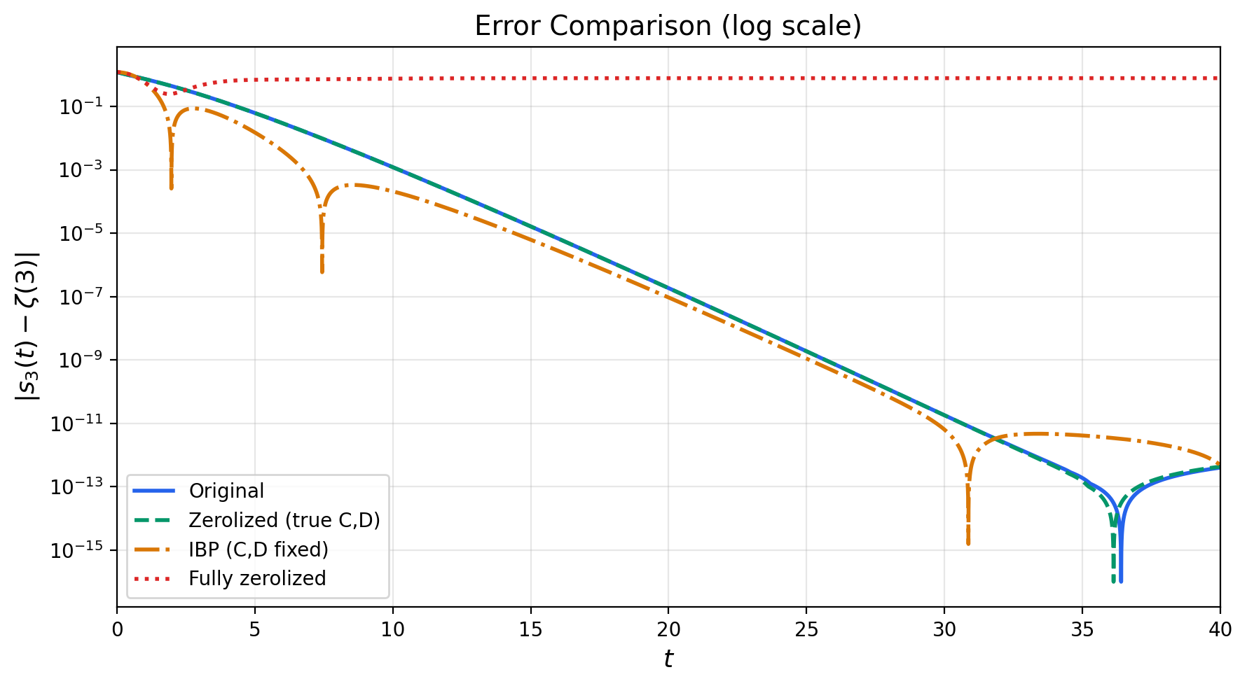
The error never decreases. The zerolized system stabilizes at a value that has nothing to do with $\zeta(3)$.
Why it fails
The problem is subtle. The E-block converges to the correct constants asymptotically, but the main system doesn’t wait. From $t = 0$, the main ODE is already evolving with the wrong coefficients (because $E_2(0) = 0 \neq C$). By the time $E_2$ gets close to $C$, the main system has already drifted to a different trajectory. The accumulated error from the transient period never washes out.
This is not a numerical issue — it’s a structural one. The main system’s dynamics at early times depend sensitively on the constants, and the auxiliary block’s convergence is too slow to catch up.
Integration by parts (IBP) can partially compensate: if the constant $C$ appears linearly in the integrand, one can replace $C$ with $E_2(t) + t \cdot \dot{E}_2(t)$, which corrects for the transient. This works when $C$ and $D$ are held fixed in the main drift. But when everything is zerolized — when $e$, $C$, and $D$ are all replaced by their dynamical estimates — the IBP trick is no longer sufficient.
The Hierarchy Question
This leads to a genuinely open question. Define:
- Level 0: Numbers computable by PIVPs with trivial initial values (rationals, or all zeros).
- Level 1: Numbers computable by PIVPs whose initial values are themselves Level 0 computable.
- Level $k$: Numbers computable by PIVPs whose initial values are Level $k-1$ computable.
Our $\zeta(3)$ construction lives at Level 1: the initial values ($e$, $\frac{1}{e-1}$) are Level 0 computable (the E-block computes them from trivial IVs), but the full system requires these computed values as inputs.
The open question: Does this hierarchy collapse?
That is: can every Level 1 number be computed at Level 0? Can you always find a single PIVP with trivial initial values that computes the same number?
If the hierarchy collapses, then the initial-value issue is purely a matter of convenience — any construction with non-trivial IVs can be rewritten with trivial ones (perhaps with more variables or slower convergence). If the hierarchy is strict, then there exist numbers that genuinely require “two stages” of ODE computation: one stage to prepare the initial values, another to compute the target.
The analogy to computational complexity is suggestive. In Turing computation, the tape starts empty and the machine does everything. But would Turing machines be strictly weaker if we added an oracle tape? That question (P vs NP, and its relativized variants) is famously open. The PIVP version — whether CRN-computable numbers form a strict hierarchy by initial-value complexity — is our analog of that question.
What we know: the hierarchy doesn’t collapse naively. You can’t just plug in dynamical estimates and expect convergence, as we showed above. Whether a cleverer construction exists is unknown.
What This Means
This isn’t just a curiosity. It demonstrates something fundamental about the relationship between computation and dynamics:
-
Polynomial ODEs are surprisingly powerful. Eight variables and eight polynomial equations are enough to compute a transcendental constant that took one of the great mathematicians of the 20th century years to prove irrational.
-
Chemistry can compute. Every term in our ODE system is at most degree 3 — well within the range of bimolecular and trimolecular reactions. In principle, this system could be implemented as a chemical reaction network.
-
The analog framework is natural for certain problems. We didn’t discretize anything. No bits, no registers, no carry chains. The computation flows continuously from $t = 0$ toward the answer. The physics of differential equations is the algorithm.
Whether anyone will actually build a chemical system that computes $\zeta(3)$ is another question. But the fact that such a system exists — that’s mathematics.
The construction here is based on classical integral representations of $\zeta(3)$ combined with the GPAC framework for polynomial ODEs. The zerolization technique for removing transcendental initial values is part of ongoing research on bounded analog complexity.
References
- R. Apéry, “Irrationalité de $\zeta(2)$ et $\zeta(3)$,” Astérisque, 61:11–13, 1979.
- C. E. Shannon, “Mathematical theory of the differential analyzer,” Journal of Mathematics and Physics, 20(4):337–354, 1941.
- O. Bournez, D. S. Graça, and A. Pouly, “Polynomial time corresponds to solutions of polynomial ordinary differential equations of polynomial length,” Journal of the ACM, 64(6):1–76, 2017. [Polynomial-time equivalence of GPAC and Turing machines.]