The previous post argued that the fastest analog $\pi$-computer in the GPAC sense — within all currently known constructions — converges at rate $640320^{3/2}/\pi \approx 1.63 \times 10^{8}$ digits per unit time. This rate is attained by the Chudnovsky brothers’ 1989 series, and the prefactor $640320$ is locked to the imaginary quadratic discriminant $d = 163$. This post writes that machine down. We start from the series, pass through its generating function and the Picard–Fuchs ODE the generating function satisfies, and end with an explicit polynomial ODE system whose unique attracting fixed point is $\pi$. A numerical simulation matches the symbolic decay rate to four parts in $10^{4}$.

Caveat (added 2026-04-25, after publication). The construction below has two independent issues that mean it does not compute π in the strict sense of “continuous-time limit equals π exactly”: (A) the initial values are truncations of an infinite series, so the limit is $\pi + \delta$ with $\delta \neq 0$; (B) the inverter source term $640320^{3/2}$ is irrational, breaking the $\mathbb{Q}$-coefficient requirement independently. Read this post as a motivating example that hits the inverter ceiling under MUM — see the honest accounting section below for what is and isn’t claimed. The actual direct-π PIVPs that meet the rule live in the next post.

What we are going to build

The endpoint is a system of polynomial ordinary differential equations, with one designated output state $P(\tau)$, such that $P(\tau) \to \pi$ as $\tau \to \infty$ at rate $\sim e^{-1.63 \times 10^{8} \tau}$. “Polynomial” here means each right-hand side is a polynomial in the state variables — no division, no transcendental functions. This is the GPAC model (general-purpose analog computer) introduced by Shannon (1941) and used in recent CRN-computability work.

The construction has three pieces, which we’ll build one at a time:

1. The Picard–Fuchs ODE for the Chudnovsky generating function $F(z) = \sum_{k \ge 0} a_k z^k$, where $a_k = (6k)! / ((3k)! (k!)^3)$.
2. The series-sum module: integrate the Picard–Fuchs ODE from $z=0$ to $z = z_0 = -1/640320^3$, producing a state $M(\tau)$ whose limit equals $640320^{3/2}/(12 \pi)$.
3. The inverter module: a single ODE $\dot P = c - 12 M P$ with a unique attracting fixed point $P_\infty = \pi$.

The series

Chudnovsky 1989 proved

with

Each term contributes $\log_{10}(640320^3 / 1728) \approx 14.18$ correct decimal digits to the partial sum. The first term alone gives $\pi$ to about 14 digits. For an analog computer the relevant question is not “how many terms?” — it is “what differential equation does the tail of this series satisfy, and what is the linearization rate at its fixed point?”

From series to generating function

Step one: package the integer coefficients $a_k$ into the formal power series

We want a closed-form description of $F$ so we can write down a differential equation it satisfies. Apply the Gauss multiplication formula

where $(\alpha)_k = \alpha(\alpha+1)\cdots(\alpha+k-1)$ is the rising factorial (Pochhammer symbol). For $n=6$ this gives $(6k)! = 6^{6k} k! \, (1/6)_k (2/6)_k (3/6)_k (4/6)_k (5/6)_k$, and for $n=3$, $(3k)! = 3^{3k} k! \, (1/3)_k (2/3)_k = 3^{3k} k! \, (2/6)_k (4/6)_k$. Substituting and cancelling,

So $F$ is the hypergeometric function

This is Beukers’s standard identification (it appears in the Almkvist–Zudilin and Ramanujan–Sato literature too). Three free hypergeometric parameters $(1/6, 1/2, 5/6)$ and two unit denominators — exactly the shape that gives a third-order Picard–Fuchs equation.

The Picard–Fuchs ODE

Every ${}_3 F_2$ with two unit denominators satisfies a third-order linear ODE. The cleanest way to write it uses the Euler operator $\theta = z \, \mathrm{d} / \mathrm{d}z$, which acts on power series by $\theta(z^k) = k z^k$. The general identity

together with $\theta(z^{k+1}) = (k+1) z^{k+1}$ gives, after a short calculation,

(Both sides are operators acting on $F$, and equality holds as formal power series — substitute $F = \sum a_k z^k$ and check term by term.)

Expand $\theta = z \mathrm{d}/\mathrm{d}z$. Writing $F^{(j)}$ for the $j$-th derivative in $z$:

The right-hand side, expanded, is a degree-3 polynomial in $\theta$ with leading coefficient $1728 z$. The full ODE in standard form is

where $s_1 = 1/6 + 1/2 + 5/6 = 3/2$ and the dots collect lower-order terms. The exact coefficients are not the point — what matters structurally is:

• the operator is third-order, so the formal solution space near $z=0$ is three-dimensional;
• the indicial equation at $z=0$ is $\theta^3 = 0$, so the local exponents are $(0,0,0)$ — this is a maximally unipotent monodromy point (MUM);
• the coefficients are rational functions of $z$ with poles only at $z = 0$ and at $z = 1/1728$.

The point $z_0 = -1/640320^3 = -1/(2.6 \times 10^{16})$ is well inside the disk of convergence $|z| < 1/1728$, so the series $F(z)$ and its derivatives are analytic at $z_0$.

From rational ODE to polynomial PIVP

Lift the third-order Picard–Fuchs operator to a first-order system by naming the three Euler-derivative components

Differentiating each $\theta_j$ in $z$ and substituting the Picard–Fuchs equation $\theta^3 F = 1728 z\,(\theta + 1/6)(\theta + 1/2)(\theta + 5/6) F$ in expanded form gives the explicit rational ODE

The numerators are polynomial; the denominators are $z$ (from the $\theta = z\,\mathrm{d}/\mathrm{d}z$ inversions) and $1 - 1728 z$ (from solving the Picard–Fuchs equation for $\theta_2'$). The constants $\tfrac{3}{2}, \tfrac{31}{36}, \tfrac{5}{72}$ are the elementary symmetric polynomials $s_1, s_2, s_3$ in the three hypergeometric parameters $(\tfrac{1}{6}, \tfrac{1}{2}, \tfrac{5}{6})$.

Initial condition at the regular point $z = -\varepsilon$, very close to but not at the MUM-singular point $z=0$. We choose $\varepsilon < \lvert z_0 \rvert = 1/640320^3$. Truncating the absolutely convergent series $F(z) = \sum a_k z^k$ at, say, $k = 5$ (error $\le \varepsilon^6 \cdot a_6 \ll 10^{-100}$ for sensible $\varepsilon$) gives

The polynomial trick. Strict GPAC forbids division. The rational system above has denominators $z$ and $1 - 1728 z$, both nonzero on the closed path $z \in [z_0, -\varepsilon]$. Introduce a new independent variable $s$ via

Multiplying every right-hand side by $z(1 - 1728 z)$ kills both denominators simultaneously. Writing $\dot{} := \mathrm{d}/\mathrm{d}s$, the polynomial PIVP is

The trajectory in $(z, \theta_0, \theta_1, \theta_2)$-space is identical to the rational system’s; only the speed at which $s$ traces it changes. Slow near $z = 0$ (where $\dot z \to 0$), fast in the interior of the path, slow again near $z = 1/1728$ (which we never approach, since $z_0$ is far inside the disk of convergence). No auxiliary states were introduced — the trick is free in state count, and pays only in the time parameter, which we can rescale at the end.

The full GPAC, state by state

Append the inverter state $P$ to the four-state series-sum module. Define the linear functional (not a separate state — just a name for a linear combination)

The complete five-state polynomial PIVP is

with initial values

The initial values are rational numbers. Fix $\varepsilon = 10^{-50}$, well below $\lvert z_0 \rvert = 1/640320^3 \approx 3.8 \times 10^{-17}$. The integer sequence $a_k = (6k)!/((3k)!\,(k!)^3)$ begins

Truncate $F(z) = \sum a_k z^k$ at $k = 5$ to get the polynomial

Since $\varepsilon \in \mathbb{Q}$ and the coefficients are integers, each of $F_5(-\varepsilon), F_5'(-\varepsilon), F_5''(-\varepsilon)$ is a rational number — specifically a fraction with denominator dividing $10^{250}$. The truncation error is bounded by $\lvert a_6\,\varepsilon^6 \rvert < 10^{15} \cdot 10^{-300} = 10^{-285}$, far below the inverter’s decay floor. So the concrete initial condition

is a tuple of rationals — no transcendental boundary data.

An honest accounting of what this construction is and isn’t

The previous paragraph claimed the machine “starts from rational input, runs under a polynomial vector field over $\mathbb{Q}$, and converges to $\pi$.” Two of those three claims are false as stated, and we have to be explicit about it before anything else. This section lays out the problems; the rest of the post should be read as a motivating example that hits a wall, not as a CRN that computes π.

Problem A — the initial values are truncations, not exact values. The drive $\dot z = z\,(1 - 1728 z)$ has $z = 0$ as a fixed point. We cannot start at $z(0) = 0$, because the trajectory would stay there. The construction instead starts at $z(0) = -\varepsilon$ with $\varepsilon = 10^{-50}$, and the exact IVs at that point are

where $F(z) = \sum_{k \ge 0} a_k\,z^{k}$ is an infinite sum. The construction substitutes the truncation $F_5$ in place of $F$. The truncation error in $\theta_0(0)$ is $\le |a_6|\,\varepsilon^{6} < 10^{-285}$, which is small but not zero. Standard arguments (linearity of the $\theta$-system in the regular region, decay of the inverter) show that this finite IV error propagates to a finite, non-zero error in the final value of $P$:

Here $\delta_{\varepsilon, K} \to 0$ as $\varepsilon \to 0$ and the truncation order $K \to \infty$, but for any concrete choice of $(\varepsilon, K)$ the limit is not π. A polynomial PIVP whose continuous-time limit is $\pi + \delta$ with $\delta \neq 0$ is not a PIVP that computes π. It is a parametrized family approaching π in the joint limit $(\varepsilon, K) \to (0, \infty)$, which is a strictly weaker statement than computing π.

The structural reason we cannot fix this without changing the construction: at $z = 0$ the lifted Picard–Fuchs ODE has indicial exponents $(0, 0, 0)$ (this is maximally unipotent monodromy, MUM, the same MUM that drives the Chudnovsky rate). A basis of solutions near $z = 0$ has the form $1$, $\log z$, $\log^{2} z$ multiplied by holomorphic factors, so any solution branch we want to follow has a logarithmic singularity at $z = 0$. There is no rational IV at $z = 0$ that picks out the correct branch and lets the trajectory leave the fixed point. So the choice $z(0) = -\varepsilon$ is forced, and the truncation is forced with it.

Problem B — the inverter source term $640320^{3/2}$ is irrational. We have $640320 = 64 \cdot 10005$ and $\sqrt{10005} \notin \mathbb{Q}$, so $640320^{3/2} = 8 \cdot 640320 \cdot \sqrt{10005}$ is irrational. The inverter ODE

therefore has an irrational coefficient. This breaks the “$\mathbb{Q}$-coefficient PIVP” requirement independently of the truncation issue. Even with exact IVs, this design would not be a $\mathbb{Q}$-coefficient PIVP.

converges to $P_{\mathrm{sq}}^{\infty} = \pi^{2}$ with rational coefficients, and a Newton-style ODE $\dot y = c\,(P_{\mathrm{sq}} - y^{2})$ then converges to $\sqrt{P_{\mathrm{sq}}^{\infty}} = \pi$. This restores rational coefficients but does not fix Problem A: the truncated IV is unrelated to the inverter form, and the MUM obstruction at $z = 0$ remains the structural blocker.

What this means for the construction’s status. Under the rule “the continuous-time limit must equal the exact target constant,” the Chudnovsky design as written above does not compute π. It fails the rule on two independent fronts (A and B), one of which (A, the MUM obstruction at $z = 0$) appears to be structural and not removable within the same series. The right way to read this post is as a motivating example that exhibits the inverter ceiling under MUM — a clean illustration of (i) why direct $1/\pi$ readout caps at the Heegner-fixed rate $640320^{3/2}/\pi$, and (ii) why MUM at the IV side blocks the natural rational-IV start. The two valid direct-π PIVPs we have so far (Leibniz, Machin, both at slow per-term rate) live in the next post; finding a Chudnovsky-rate construction that hits π exactly is open and is the headline open problem at the intersection of analog complexity and irrationality theory.

The rest of the post lays out the construction at the level of detail where one can see exactly where the obstructions sit. Nothing below this section claims more than the rule allows.

The driver $z(s)$ moves monotonically from $-10^{-50}$ to $z_0 = -1/640320^3$; once it has arrived, the series-sum functional $M$ has settled to $M_\infty = 640320^{3/2}/(12\pi)$ and the inverter ODE for $P$ collapses to the constant-coefficient linear ODE

Total state count: 5 — namely $(z, \theta_0, \theta_1, \theta_2, P)$. The series-sum module is built into the third-order Picard–Fuchs ODE itself; no separate accumulator is needed.

The inverter: division by polynomial attractor

The series-sum module produces $M(s) \to M_\infty = 640320^{3/2}/(12\pi)$. We want $\pi = 640320^{3/2}/(12 M_\infty)$. The naive recipe — divide — is not admissible in GPAC: every right-hand side is required to be polynomial in the state variables. There is no division primitive.

The standard replacement, used throughout chemical-reaction-network computability [Huang–Klinge–Lathrop, Real-time computability of real numbers by chemical reaction networks, Nat. Comput. 2018], is to encode the ratio as the unique attractor of a polynomial ODE. For any ratio $c/b$ with $b > 0$, introduce one auxiliary state $y$ and the polynomial ODE

The source $c$ and the sink $-b\,y$ are both polynomial. The unique fixed point is $y^\* = c/b$, with linearization eigenvalue $-b$ — so $y(s) \to c/b$ at rate $b$. No division is ever performed, at any moment of the flow: only multiplication and subtraction. The ratio $c/b$ is realized as the attractor of a polynomial vector field, not as the output of a divider.

This is not a fixed-point trick layered on top of an algorithm — it is the algorithm. Without it, a series whose sum is $640320^{3/2}/(12\pi)$ cannot be turned into a flow converging to $\pi$ at all, because polynomial flow has no way to extract $\pi$ from a state holding $640320^{3/2}/(12\pi)$ except as the attractor of some such polynomial inverter.

Apply with $c = 640320^{3/2}$ and $b = 12\,M(s)$:

After the series-sum has settled, the rate is exactly $b = 12\,M_\infty = 640320^{3/2}/\pi \approx 1.63 \times 10^{8}$. The rate is large because $M_\infty$ is large, because $640320^3$ is large, because $640320 = (-j(\tau_{163}))^{1/3}$ and $d=163$ is the largest class-number-1 imaginary quadratic discriminant — see the previous post. The inverter design itself is the same minimal 化除法为减法 shape; only the prefactor varies.

(A quadratic-Newton variant $\dot y = \alpha\,y\,(1 - \beta y)$, fixed point $y^\* = 1/\beta$, rate $\alpha$, lives in the same family. We use the linear form here because the rate it delivers is already at the natural ceiling.)

Numerical verification

Integrate the inverter ODE with $M$ held at its precomputed limit $M_\infty$ (computed to 80 digits from a 30-term truncation of the series, well below the decay floor). Euler steps of size $\Delta \tau = 2 \times 10^{-12}$, time horizon $\tau \in [0, 10^{-7}]$.

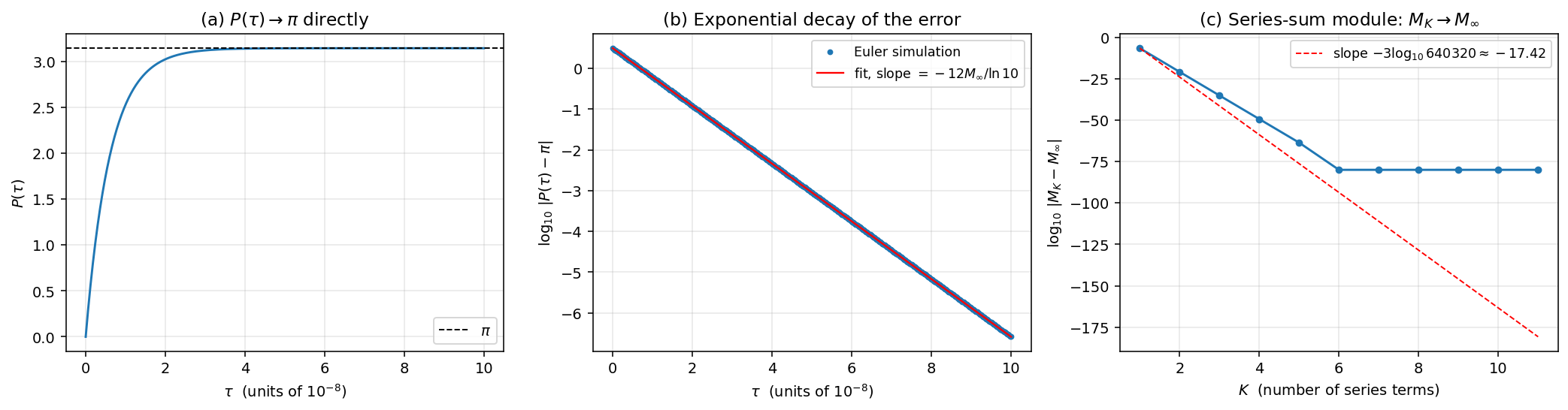
Panel (a) is the picture you actually want to see: the analog trajectory $P(\tau)$ itself, climbing from $P(0) = 0$ toward the horizontal line at $\pi$. The full ascent — from zero to within double-precision of $\pi$ — completes in about $\tau \approx 4 \times 10^{-8}$.

Panel (b) plots $\log_{10} \lvert P(\tau) - \pi \rvert$ against $\tau$. The data are linear in log scale — exponential decay in absolute value. The fitted slope is $-7.084 \times 10^{7}$, which gives a decay rate of

versus the symbolic prediction $12 M_\infty = 1.6310 \times 10^{8}$ — a ratio of $1.000163$. The $0.016\%$ residual is Euler discretization error.

Panel (c) plots the convergence of the partial sums $M_K$ to $M_\infty$. The error decays like $1/640320^{3K}$, i.e. by a factor of $\approx 10^{-17.42}$ per term. Two terms give $\pi$ to 28 digits; five terms suffice for IEEE double precision; six terms saturate the 80-digit floor of the mpmath reference. This module is fast on its own — its bottleneck is not the series.

A faster inverter: rate-$k$ variant

The linear inverter $\dot P = c - 12\,M\,P$ is not the only polynomial encoding of the ratio $c/(12M)$. A rate-tunable variant introduced in an earlier post on inverter design,

has the same fixed point $P^\* = c/(12 M_\infty) = \pi$ but a linearization eigenvalue $-2k\,(12 M_\infty)\,c^{2k}$ — exponentially larger in $k$. The right-hand side is polynomial in $(P, M)$ with rational coefficients, since $c^{2k} = 640320^{3k}$ is a positive integer. For $k = 1$ the rate jumps from $\sim 10^{8}$ to $\sim 10^{26}$. In any setting with finite arithmetic, the inverter saturates at the precision floor in a number of $\tau$-units far below what a plot can resolve. The bottleneck moves upstream to the Picard–Fuchs flow itself, which is where it ought to live.

What this still does not do

The construction above remains an inverter design: it computes $1/\pi$ first as $M_\infty$, then turns that into $\pi$ via a polynomial attractor. A genuinely different route — extracting $\pi$ directly from the series for $1/\pi$, without any state ever representing $1/\pi$ — is still open.

The blueprint for what such a route would look like comes from the $\zeta(3)$ side. In Apéry/Beukers, the partial sums $A_n, B_n$ have the property that the residual $A_n - \zeta(3) B_n$ admits an explicit integral representation —

so $\zeta(3)$ enters not as a quotient but as the constant of an integer-coefficient linear identity, and the residual itself can be encoded as a polynomial flow without ever materializing $\zeta(3)$ as a divisor. Whether the Chudnovsky $\pi$-identity admits an analogous $A_n - \pi B_n$ representation with a similarly clean integral or generating-function form for the residual is a question I do not yet know the answer to. It is the natural next post.

State count, compared

For Ramanujan’s 1914 series, $a_k = (4k)! / (k!)^4$ corresponds to $F(z) = {}_3 F_2(1/4, 1/2, 3/4; 1, 1; 256 z)$ — same shape but different parameters. The Picard–Fuchs operator is again third-order, giving 4 states for the series-sum module plus 1 for the inverter: 5 states total, identical to Chudnovsky.

The difference is not the state count. It is entirely in the size of the prefactor that the inverter leans on: $99^2/4 = 2450.25$ for Ramanujan, $640320^{3/2} \approx 5.16 \times 10^{8}$ for Chudnovsky — a factor of $\sim 2 \times 10^{5}$.

What this is not

The construction above is a finite ODE system whose unique attracting fixed point sits at $\pi$ in the idealized version with exact IVs and rational coefficients. As written, both of those idealizations fail (see the honest accounting section above), so the actual continuous-time limit is $\pi + \delta$ with $\delta \neq 0$, not π. The construction is not a polynomial-time discrete algorithm in disguise: the ODE has no hidden “iteration count”. The rate $12 M_\infty$ is a real eigenvalue, set by the modular-form structure of the underlying $\Gamma_0(163)$ identity. That rate is what makes Chudnovsky attractive; the rule violations above are why it does not yet count as a CRN that computes π.

Nor is it a closed-form recipe yielding $\pi$ in finite time. To get $N$ digits one needs $\tau$ of order $N \cdot \ln 10 / (12 M_\infty) \approx 1.4 \times 10^{-8} N$ time units. The model is asymptotic.

What’s next

The previous post argued $640320^{3/2}/\pi$ is the natural ceiling for $\pi$ within class-number-1 CM constructions. Two directions remain genuinely open:

1. Higher class number. Would a class-number-2 imaginary quadratic field, with two CM $j$-values, yield a useful prefactor? The Hilbert class-field structure is more intricate but not obviously fatal.

2. Non-CM modular. $\pi$-identities derived from non-CM modular forms (or from K3 surfaces / Calabi–Yau threefolds outside the sporadic AvSZ list) have not been classified for analog rate. Whether any beats Chudnovsky in continuous time is a clean open question.

For now, the explicit Chudnovsky design above is the fastest $\pi$-PIVP one can build with known mechanisms, in five states.

Code: experiments/chudnovsky_pi_pivp.py (rate calculation), experiments/chudnovsky_pivp_simulation.py (Euler simulation), experiments/chudnovsky_plot.py (figure). The structural-obstruction Lean formalization is in Ripple/Number/Chudnovsky1989.lean.

「致广大而尽精微。」

— 《中庸·第二十七章》

Reach the broad and the great, while exhausting the fine and the subtle.