How Hard Is It to Compute α^β? A Bounded GPAC Error Analysis
2026-04-01
The Question
Suppose you have two real numbers, $\alpha > 0$ and $\beta$, each computable by a bounded analog system (a GPAC — General-Purpose Analog Computer). You know how hard each one is to compute: $\alpha$ takes time $\mu_\alpha(r)$ to get $r$ bits of precision, and $\beta$ takes $\mu_\beta(r)$.
How hard is it to compute $\alpha^\beta$?
This question sits at the intersection of computable analysis and analog complexity theory. The answer turns out to be surprisingly clean.
The Construction
The identity $\alpha^\beta = e^{\beta \ln \alpha}$ suggests a plan: compute $\ln \alpha$, multiply by $\beta$, exponentiate. In the GPAC world, this becomes a system of polynomial ODEs. The key trick is to avoid the singularity of $\ln(x)$ at $x = 0$ by working with $\ln(1 + x_1)$ where $x_1 \to \alpha - 1$ starts from zero.
The construction uses four variables:
with $x_1(0) = u(0) = v(0) = 0$ and $z(0) = 1$, where $x(t) \to \alpha$ and $y(t) \to \beta$ are provided by upstream GPACs.
At equilibrium: $x_1 \to \alpha - 1$, $u \to \ln\alpha$, $v \to (\alpha - 1)/\alpha$, and — here’s the beautiful part — the ODE for $z$ is equivalent to $z(t) = e^{y(t) \cdot u(t)}$, so $z \to e^{\beta \ln \alpha} = \alpha^\beta$.
The Error Analysis
Since this is a GPAC (not a CRN), we can do standard computable analysis error propagation — no dual-railing, no subtraction modules, no readout overhead. The analysis has four clean steps.
Step 1: The tracking filter
The variable $x_1$ tracks $\alpha - 1$ through the ODE $e_1' + e_1 = (x(t) - \alpha)$, where $e_1 = x_1 - (\alpha - 1)$. This is a first-order low-pass filter with cutoff frequency 1.
The convolution gives:
If $\varepsilon_\alpha(t)$ decays slower than $e^{-t}$ (sub-exponential convergence), the filter is transparent: $|e_1(t)| \sim \varepsilon_\alpha(t)$. The tracking step preserves the complexity class of $\alpha$.
Step 2: Logarithm and ratio errors
Since $u = \ln(1 + x_1)$ and $v = x_1/(1 + x_1)$, the mean value theorem gives errors proportional to $|e_1(t)|$ with constant factors depending on $\alpha$. No new dynamics, no additional slowdown.
Step 3: The exponent
The exponent $R(t) = y(t) \cdot u(t)$ targets $\beta \ln \alpha$. The triangle inequality splits the error into two terms:
One term comes from the $\beta$-error, the other from the $\alpha$-error. Each carries a constant factor.
Step 4: The output
The mean value theorem on $e^x$ gives the final error:
The Result
Theorem (Complexity of $\alpha^\beta$). If $\alpha > 0$ and $\beta$ are computable by bounded GPACs with time moduli $\mu_\alpha(r)$ and $\mu_\beta(r)$, then $\alpha^\beta$ is computable with time modulus
$$\mu_{\alpha^\beta}(r) = \max\!\big(\mu_\alpha(r + C),\; \mu_\beta(r + C)\big) + O(1),$$where $C$ depends only on $\alpha$ and $\beta$.
In words: the complexity of $\alpha^\beta$ is the harder of the two inputs, up to a constant shift in precision. Exponentiation does not change the complexity class.
Examples
| $\alpha$ | $\beta$ | $\mu_\alpha$ | $\mu_\beta$ | $\mu_{\alpha^\beta}$ |
|---|---|---|---|---|
| $\pi/4$ | $e$ | $\Theta(r)$ | $\Theta(r)$ | $\Theta(r)$ |
| algebraic | $e$ | $\Theta(r)$ | $\Theta(r)$ | $\Theta(r)$ |
| $\alpha$ (poly-time) | $\beta$ (linear) | $\Theta(r^k)$ | $\Theta(r)$ | $\Theta(r^k)$ |
Since $\pi$ and $e$ are both computable in linear time by known GPAC constructions, $(\pi/4)^e \approx 0.5186$ is also computable in linear time.
Why This Is Nice
Three things make this analysis satisfying:
-
No CRN overhead. Because we stay in the GPAC model (which handles signed values natively), there’s no dual-railing, no subtraction module, no readout. The error analysis is pure computable analysis.
-
The low-pass filter shows up again. The $x_1$ tracking ODE $e_1' + e_1 = \text{input error}$ is mathematically the same first-order low-pass filter that appears in CRN readout modules (see my post on CRN subtraction as a low-pass filter). But here it arises naturally within the GPAC construction, not from a CRN compilation step.
-
The answer is what you’d hope. In computable analysis, computing $f(x, y)$ from approximations to $x$ and $y$ typically costs the max of the two input precisions, plus overhead depending on the Lipschitz constant of $f$. That’s exactly what we get: the constant $C$ absorbs $\alpha^\beta$, $|\ln\alpha|$, and $|\beta|$, and the time modulus is the max.
Full System Simulation: $(\pi/4)^e$
Here is the complete GPAC system in action. Both inputs ($\alpha(t) \to \pi/4$ and $\beta(t) \to e$) converge exponentially, and we simulate all four internal variables.
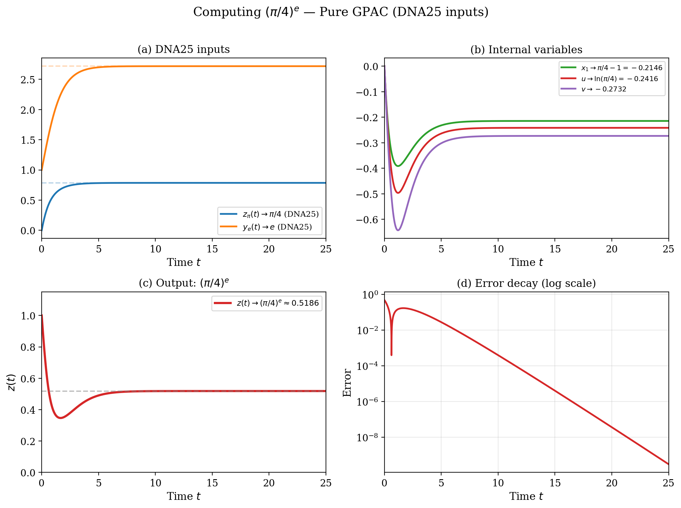
(a) The two input components converge to their targets. (b) The internal variables: $x_1 \to \pi/4 - 1 \approx -0.215$ (negative — fine for GPACs), $u \to \ln(\pi/4) \approx -0.242$, and $v \to (\pi/4 - 1)/(\pi/4) \approx -0.273$. (c) The output $z(t)$ drops from $z(0) = 1$ to $(\pi/4)^e \approx 0.5186$. (d) Error decay on log scale (see note below): exponential convergence, confirming $\mu(r) = \Theta(r)$.
A note on log-scale error plots. Throughout this post, error plots use a logarithmic vertical axis. On a log scale, the $y$-axis shows the order of magnitude of the error: each grid line represents a factor of 10 (or $e$). An error of $10^{-4}$ appears halfway between $10^{-3}$ and $10^{-5}$.
Why use log scale? Because we care about how many bits of precision we gain per unit time. If the error decays as $e^{-ct}$ (exponential convergence), then $\log|error| \approx -ct$: a straight line on the log plot, with slope $= -c$. A steeper line means faster convergence. This is exactly the time modulus: the time to reach precision $e^{-r}$ is $t \approx r/c$, i.e., $\mu(r) = \Theta(r)$ (linear time).
In contrast, polynomial convergence ($|error| \sim t^{-k}$) would curve downward on a log plot, never becoming a straight line. The error plots in this post show straight-line behavior, confirming that our constructions achieve exponential convergence — linear time in computable analysis terms.
Full System Simulation: $e^\pi$
The same construction handles larger targets.
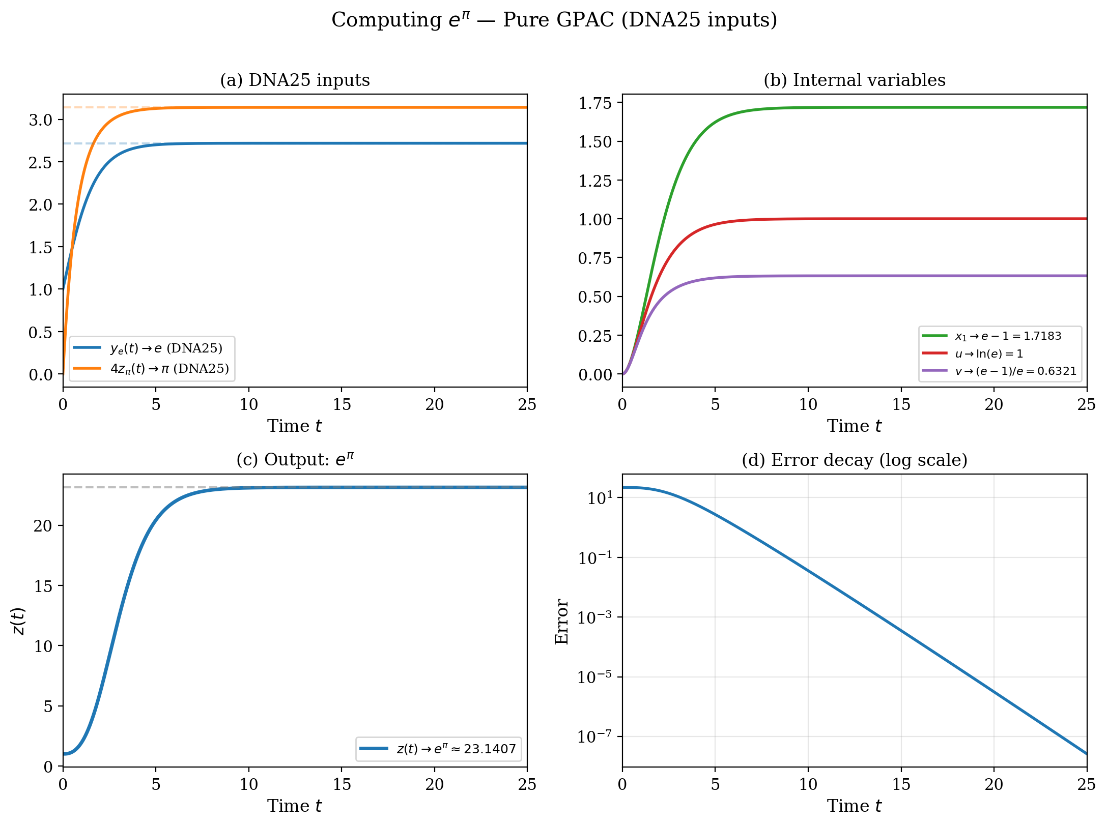
(a) Inputs converge to $e$ and $\pi$. (b) Internal variables: $x_1 \to e - 1 \approx 1.718$, $u \to \ln e = 1$ (exact!), $v \to (e-1)/e \approx 0.632$. (c) The output $z(t)$ grows from $1$ to $e^\pi \approx 23.14$. (d) Error decay: again exponential, again $\mu(r) = \Theta(r)$.
Note: $u \to \ln e = 1$ exactly — the logarithm of $e$ is the simplest possible case. The construction doesn’t “know” this; the ODE just happens to produce $u = 1$ at equilibrium.
The $(\pi/4)^e$ example is particularly interesting because $\pi/4 < 1$, so the intermediate variables $x_1$, $u$, and $v$ are all negative. This is perfectly fine in the GPAC formulation, which handles signed values natively. A CRN implementation would require dual-railing, but the complexity analysis remains the same.
Anatomy of the Error: Why the Dip?
If you look at the error plot for $(\pi/4)^e$, there’s a curious feature: the error drops sharply around $t \approx 0.6$, then rises again before settling into monotone exponential decay. This is not a numerical artifact — it’s a genuine error cancellation caused by the interplay of two competing errors.
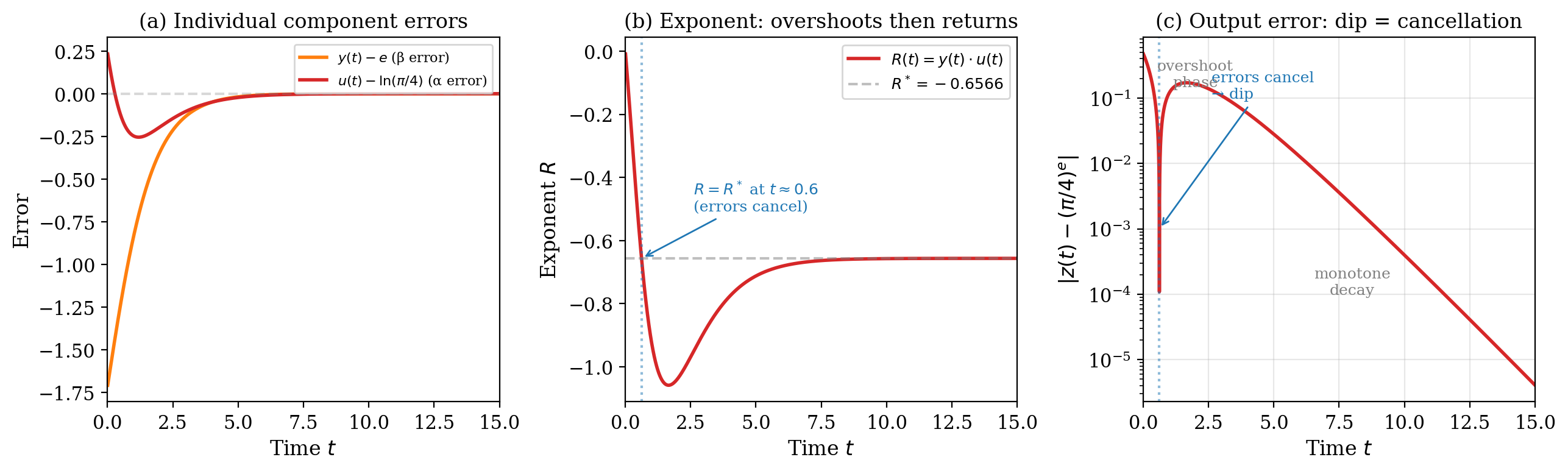
The key is that $\ln(\pi/4) \approx -0.242$ is negative. The exponent $R(t) = y(t) \cdot u(t)$ is the product of two quantities converging at different rates:
- $y(t) \to e$ from below (starts at $1$, monotonically increasing)
- $u(t) \to \ln(\pi/4) \approx -0.242$ from above (starts at $0$, goes negative)
These two errors push $R(t)$ in opposite directions:
- $y(t) < e$ makes $|R(t)|$ smaller (a smaller multiplier times a negative $u$)
- $|u(t)| > |\ln(\pi/4)|$ makes $|R(t)|$ larger (the $u$-error overshoots)
At $t \approx 0.6$, these two effects exactly cancel: $R(t) \approx R^* = e \cdot \ln(\pi/4)$, even though neither $y$ nor $u$ is close to its limit. The output $z(t) = e^{R(t)}$ passes through the target value, producing the dip.
After this moment, the $u$-error dominates (it overshot further), pushing $R(t)$ below $R^*$. Then both errors decay, and $R(t)$ returns to $R^*$ from below — producing the overshoot phase before the final monotone convergence.
This phenomenon only occurs when $\ln \alpha < 0$ (i.e., $\alpha < 1$): the two input errors push the exponent in opposite directions. For $e^\pi$ (where $\ln e = 1 > 0$), both errors push $R$ in the same direction, and the convergence is monotone.
A small but beautiful illustration of how signed intermediate quantities create error dynamics that unsigned CRN systems never see.
Simulation Code
Run it yourself — no install needed:
![]()
The notebook includes both examples, all plots, and a “Try Your Own” cell where you can plug in any $\alpha$ and $\beta$. Source code also on GitHub.
Closing Thoughts
It’s a small result, but it illustrates something important: bounded GPAC complexity composes the way you’d want it to — like computable analysis, not like a machine model with overhead at every step.