CRN Subtraction Is a Low-Pass Filter
2026-04-01
The Problem: Reading Out a Difference
Chemical reaction networks (CRNs) compute with non-negative concentrations. But when we compile a GPAC (General-Purpose Analog Computer) into a CRN, variables that can be negative get split into dual-rail pairs: $x = X^+ - X^-$ with $X^+, X^- \ge 0$. The algebraic difference $X^+ - X^-$ satisfies the original ODE exactly — the annihilation terms cancel upon subtraction.
But here’s the catch: $X^+ - X^-$ is not a single species. You can’t measure it directly in a test tube. You need a dedicated readout species $Z$ that dynamically converges to $\alpha = X^{+*} - X^{-*}$ using only mass-action reactions.
The question is: does the readout step slow down the computation?
The answer, perhaps surprisingly, comes from signal processing.
Two Subtraction Modules
There are two principal approaches to CRN subtraction.
Anderson–Joshi absolute-difference module
Anderson and Joshi (2024) design a module using three reactions:
where $A = X^+$ and $B = X^-$. Under mass-action kinetics, this gives the ODE:
Their key result: this module has input-independent speed $\ge 1$, meaning it converges exponentially regardless of the input values.
Two-reciprocal method
An earlier approach (Huang, Klinge, Lathrop, Real-time Equivalence of Chemical Reaction Networks and Analog Computers, DNA 25, 2019) uses two sequential inversions:
with $Y^* = 1/\alpha$ and $Z^* = \alpha$. This computes the difference by taking the reciprocal of the reciprocal.
The Low-Pass Filter View
Here’s the key insight. Linearize the Anderson–Joshi module around the equilibrium $Z^* = \alpha$ by writing $Z(t) = \alpha + \delta(t)$ and $x_1(t) = \alpha + \epsilon(t)$:
This is the defining equation of a first-order low-pass filter with cutoff frequency $\alpha$ and impulse response $h(t) = \alpha e^{-\alpha t}$. The readout error is the convolution:
If you’ve seen low-pass filters in signal processing, the implications are immediate:
-
Slow signals pass through unchanged. If the input error $\epsilon(t)$ decays slower than $e^{-\alpha t}$, the filter is transparent: $\delta(t) \sim \epsilon(t)$. The readout inherits the input’s convergence profile with no slowdown.
-
Fast signals get throttled. If the input converges faster than $e^{-\alpha t}$, the filter limits the output to its own intrinsic rate $e^{-\alpha t}$.
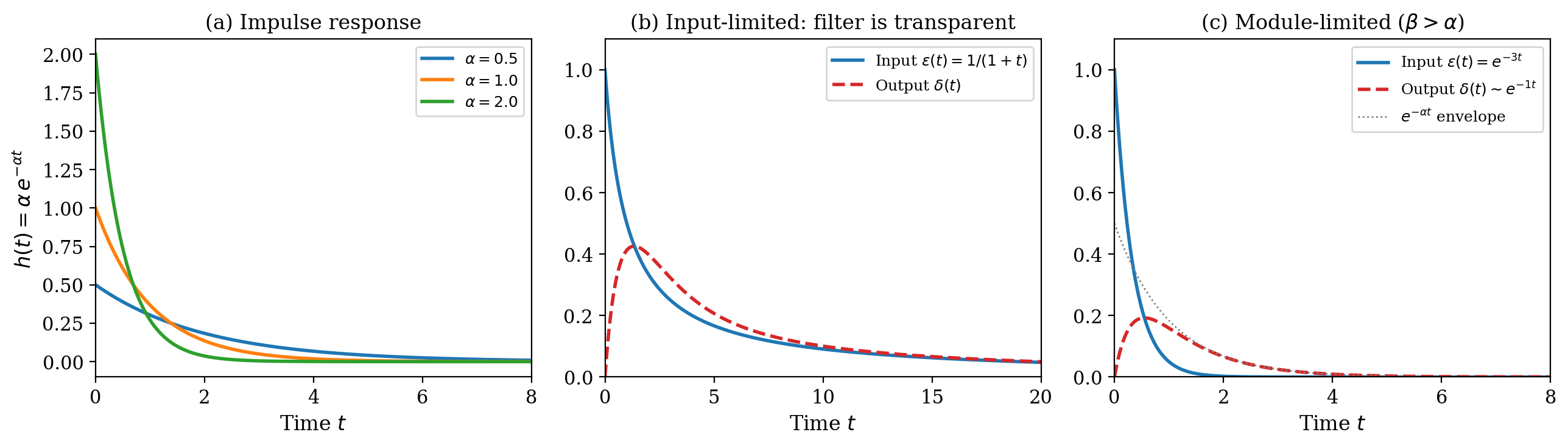
(a) Impulse responses for different cutoff frequencies $\alpha$. (b) Input-limited regime: a sub-exponential input ($1/(1+t)$, blue) passes through the filter almost unchanged (red dashed). The filter is transparent. (c) Module-limited regime: a fast exponential input ($e^{-3t}$, blue) gets throttled to the filter’s own rate $e^{-t}$ (red dashed, gray envelope).
The Two Regimes in Action
For the two-reciprocal method, linearization gives a cascade of two filters: the first inversion has intrinsic speed $\alpha$, the second has speed $1/\alpha$. The cascade’s effective speed is $\min(\alpha, 1/\alpha)$ — which is always $\le 1$, and can be very slow when $\alpha$ is large.
This is a concrete difference between the two methods: the Anderson–Joshi module has speed $\alpha$ (which can be $> 1$), while the two-reciprocal cascade has speed $\min(\alpha, 1/\alpha)$ (which is at most $1$, and drops to $0$ as $\alpha \to \infty$ or $\alpha \to 0$).
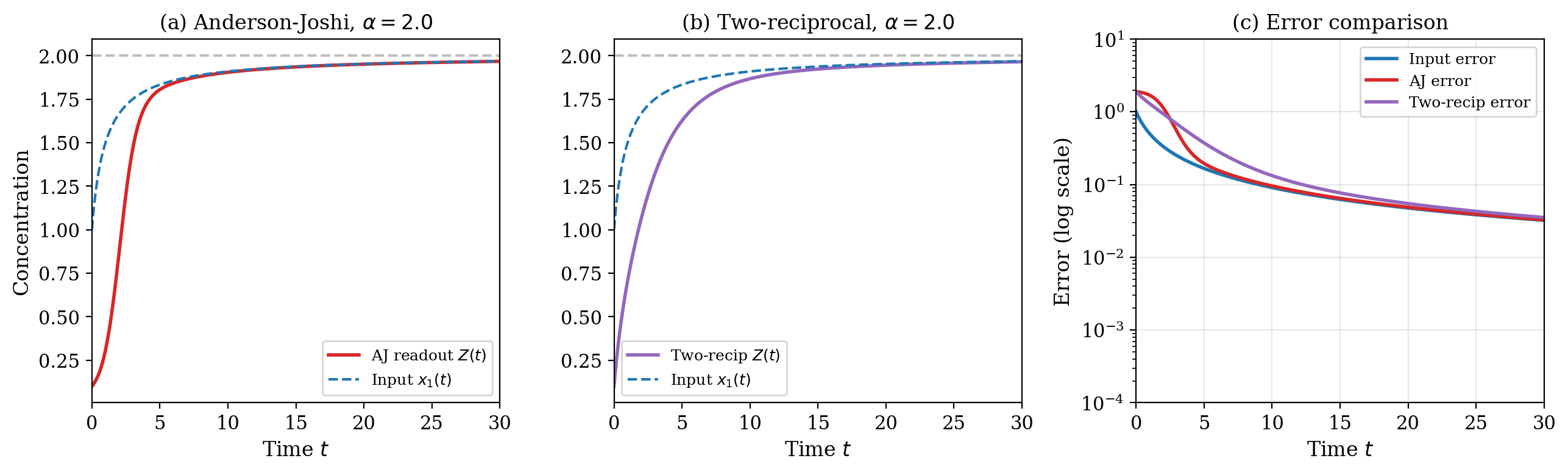
(a) Anderson–Joshi module tracking a sub-exponentially converging input ($x_1(t) \to 2$). The readout $Z(t)$ follows closely. (b) Two-reciprocal method on the same input. It also converges, but the cascade introduces a longer transient. (c) Error comparison on log scale. Both methods track the input error (blue) closely for this sub-exponential input — the filter is transparent in both cases.
The Preservation Theorem
This gives us a clean result:
Theorem (CRN readout preserves time complexity). Let a bounded GPAC compute $\alpha > 0$ with time modulus $\mu(r)$. The readout species $Z$ (via either method) satisfies:
-
If $\mu(r) = \omega(r/\alpha)$ (input slower than the filter), then $\mu_Z(r) = \mu(r) + O(1)$. Complexity preserved exactly.
-
If $\mu(r) = O(r/\alpha)$ (input at least as fast as the filter), then $\mu_Z(r) = r/\alpha + O(1)$. Throttled to linear time.
For all the constructible complexity classes we care about (computing $\alpha = 1$ at sub-exponential rates), Case 1 applies: the readout is transparent, and the CRN has the same time complexity as the GPAC.
| Class | GPAC modulus | CRN readout modulus |
|---|---|---|
| Linear | $\Theta(r)$ | $\Theta(r)$ |
| Lambert $W$ | $\Theta(r \log r)$ | $\Theta(r \log r)$ |
| Polynomial degree $n$ | $\Theta(r^n)$ | $\Theta(r^n)$ |
The Pathological Case: Computing Zero
When $\alpha = 0$, the linearization degenerates — the filter has zero cutoff frequency. The full nonlinear analysis (via Bernoulli substitution) shows:
This is polynomial convergence in ODEs, which means exponential time in computable analysis: $\mu_Z(r) = \Theta(e^r)$, regardless of how fast the input converges.
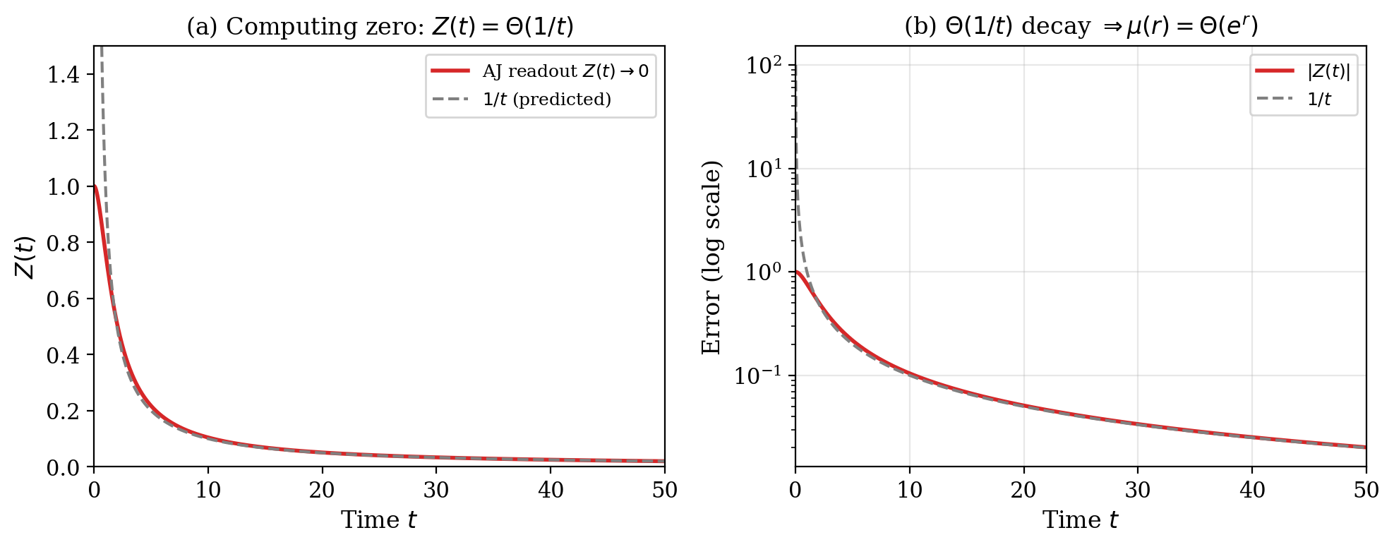
(a) The readout $Z(t)$ converges to $0$, but only as $1/t$ — agonizingly slow. (b) On log scale, the $1/t$ decay is clearly sub-exponential. To get $r$ bits of precision takes time $e^r$.
Computing zero via subtraction is fundamentally harder than computing any positive value. This is a structural limitation of the module design, not of CRNs in general — you could always build a system where a species decays directly to zero, bypassing subtraction.
The two-reciprocal method is even worse here: $Y^* = 1/\alpha \to \infty$, so it’s completely undefined at $\alpha = 0$.
Why This Matters
The low-pass filter perspective gives a unified way to reason about convergence through CRN modules. Instead of analyzing each module’s nonlinear dynamics separately, you linearize, read off the cutoff frequency, and apply the standard filter dichotomy: slow signals pass, fast signals get throttled.
This same filter structure appears in other contexts too — for instance, the $x_1$ tracking ODE in the $\alpha^\beta$ construction is mathematically identical, with cutoff frequency $1$.
The punchline: CRN subtraction doesn’t change the complexity class for any computation where the input converges sub-exponentially. The readout module is a filter, and the filter is transparent to the signals we care about.